A Basic Vocoder Tutorial, Part 1
Vocoders can be an insane amount of fun. At the root of the vocoder effect we know and love, we take an audio signal such as a human voice and use it to excite the production of another sound, such as a synthesizer. In this classic case, you may get a robotic voice effect as a result. But don't stop there. The patient explorer will discover plenty of other creative applications.
In this series, we create a vocoder with Max using the MC objects introduced in Max 8.
Patching in Max with MC
Before we jump into the vocoder itself, let's talk about MC for a moment. Just what is MC?
While it's true that the name MC was inspired by the idea of patch cords being "multi-channel", there
are countless things you can do with MC that we might not traditionally consider as "channels". So
yes, in MC you can have one patchcord carrying both the left and right channels of a stereo signal.
And yes, in MC you can have one patchcord carrying 8 channels of audio from a 7.1 surround mix.
But you can also have one patchcord that carries each band of audio frequencies in a multi-band
compressor.
For the vocoder, we will use MC both as multi-channel in the classic sense (we will ultimately create a
stereo vocoder) but we will also use MC in the multi-band sense where each "channel" of the
patchcord represents a band of audio within the "channel". If that seems challenging to wrap your
head around, don't give up! The patching will bring it to life, I promise.
Real-Time Analyzer
A real-time analyzer - or RTA - is a device that displays the spectrum of an audio signal. You could think
of it as being like a graphic equalizer, but without the equalizer. Instead, it just displays what
frequencies are actually there in each band of audio.
Like an equalizer, an RTA typically divides the spectrum up logarithmically. That sounds all fancy and
mathy, but what it means is that the bands are spread across the domain in a way that sounds even
to the human ear. For example, each band might represent 1/3 of an octave over some number of
octaves. This is in contrast to the way the FFT works, which splits audio into bands but does so
linearly rather than logarithmically. The result is that the RTA, at least the way we will build it, will use
audio bands that are more "musical" than what is produced by the FFT.
(If you are interested in the FFT, be sure to check out the series I created on that subject)
The reason we are talking about the real-time analyzer is that our vocoder will be built from the
same building blocks as an RTA. In this first installment of the series, we will create an RTA. In part 2, we will take two RTAs and combine them to make a vocoder.
Splitting the Bands
The first step to creating the RTA is to take our single audio signal and split it up into a series of
bands of audio. The basic bandpass filter in Max is called reson~, and it is the easiest tool to use for the job. Let's imagine that we want to split the signal into 20 bands. One way to do that is with 20 reson~ objects, each with a different frequency.
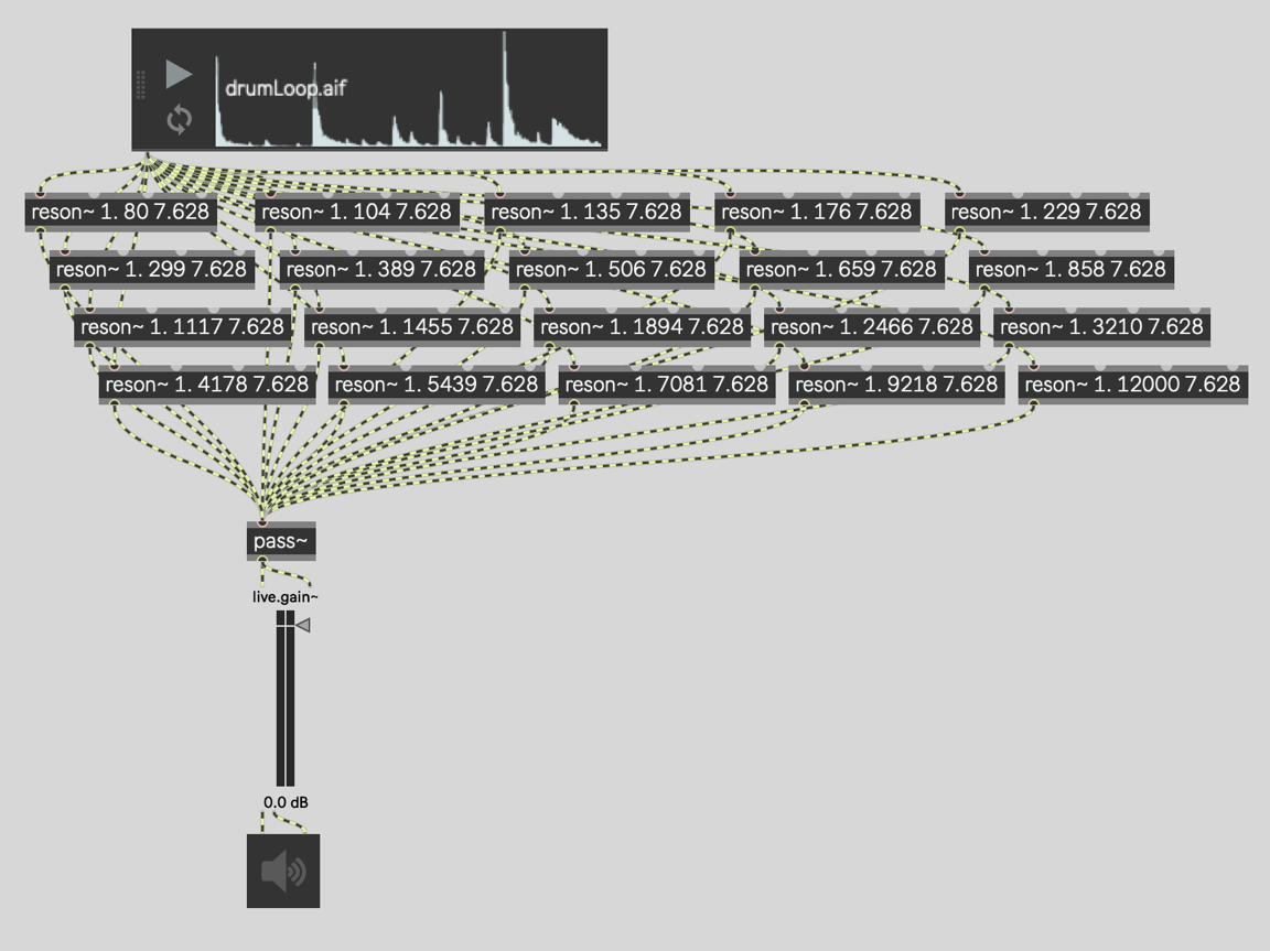
The first argument to reson~ is the gain, which is 1.0 for all of the filters, meaning there is no change or attenuation of the signal in the pass band of the filter. The second argument is the frequency, which is different for each filter. We will look at where those numbers came from later. The Q factor is always 7.628, which we will also look at later.
All of the filters are then summed at a pass~ object. This is my favorite way to sum signals together. Not only is the pass~ object the most computationally efficient object to use, but it also ensures that
if I later move this patcher into an abstraction, and then mute it using the mute~ object, that it will work as expected.
Patching together 20 reson~ filters like this isn't particularly complicated. On the other hand, it is a
pain to have to patch all of those filters together. It's even more of a pain if you want to change the
number of bands to say, 16. Or 32. Or any other number. You would, in fact, need to create entirely
separate patchers for each and every configuration!
Splitting the Bands... With MC
Most audio objects in Max can be made to handle multiple channels by using the mc. prefix on the object name. This is true of the reson~ object, which becomes mc.reson~ in the patcher below. We want 20 instances of the reson~ object, which means 20 channels of audio processing, so we add the @chans attribute to say so.
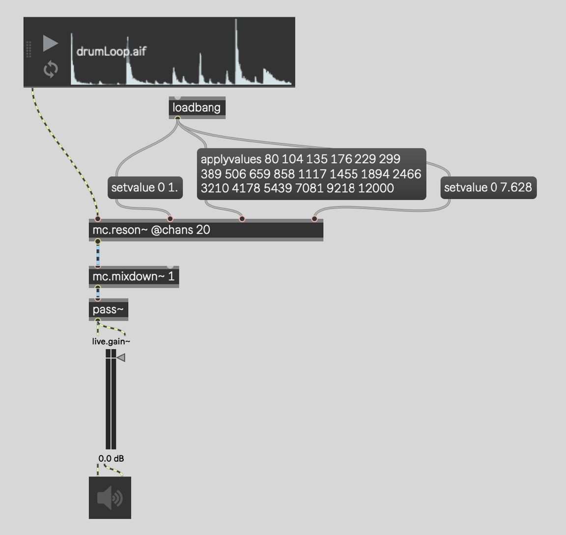
In this case, we use loadbang to set all of the gains 1.0 using the "setvalue" message. All of the Q
factors are set to 7.628 also using the "setvalue" message. We set the frequencies for all 20 filters
using the "applyvalues" message.
In MC, "setvalue" takes a list. The first number is the channel number / voice number / band number,
beginning at 1. If you specify channel/voice/band 0 then the value is applied to each and every
instance inside. In this case, there are 20 instances of a reson~ object inside.
The "applyvalues" works a little differently. Each value in the list is applied to the channel/voice/band
at each successive index in sequence. The result, in this case, is the first reson~ getting a frequency of 80 hertz, the second reson~ getting as frequency of roughly 104 hertz, and so on.
The patchcord coming out of mc.reson~ is both a different color than the signal patchcord coming in and also
wider. This is an MC patchcord and it is carrying 20 channels of audio!
The mc.mixdown~ takes those 20 channels of audio and produces another MC patchcord. This new
patchcord only has 1 channel of audio inside of it because the argument to
mc.mixdown~ is 1.
The pass~ object is not an MC object. But all of the classic Max audio objects accept MC patchcords.
When they process audio they take the first audio channel only and then discard the rest. In this case
there is only one channel so nothing is lost.
Let's Make it an RTA!
All we need to visualize our 20 bands of audio is a live.meter~ object. Contrary to what I just said about classic Max audio objects discarding all but the first channel, some objects simply adapt to the MC patchcord that connects to them. This is mostly true of UI objects that have an audio input but no audio output.
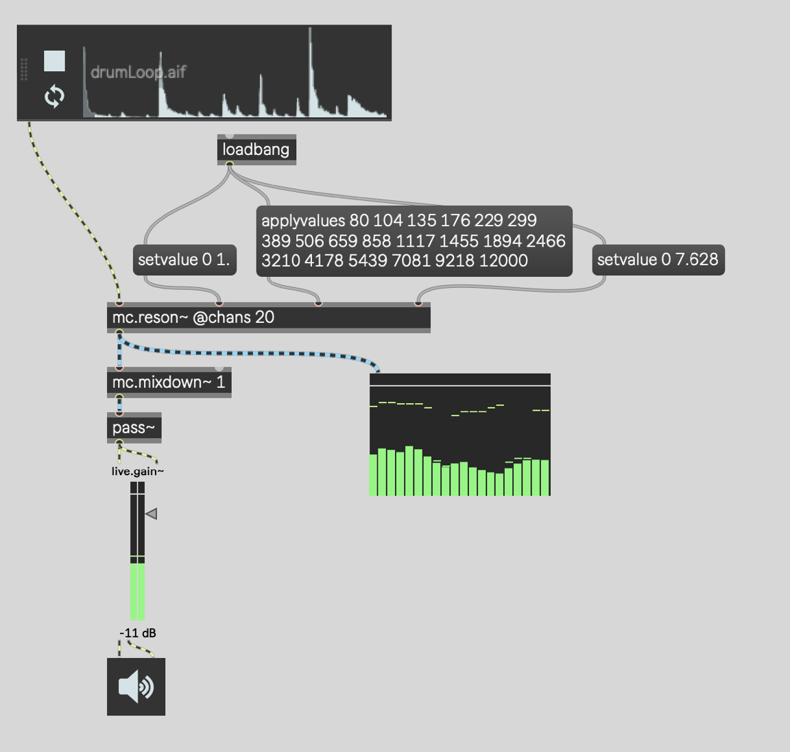
So look at that! We have a working 20-band RTA!
The only problem now is that we are stuck with a bunch of frequencies and a Q-factor that we've
accepted on faith. What if we want to change the range of frequencies or the number of bands?
Magic isn't going to cut it. We need to be able to calculate those values for ourselves.
Doing the Calculations
Let's say we want to figure out the frequencies for splitting up the audio between 80 hz and 12000 hz
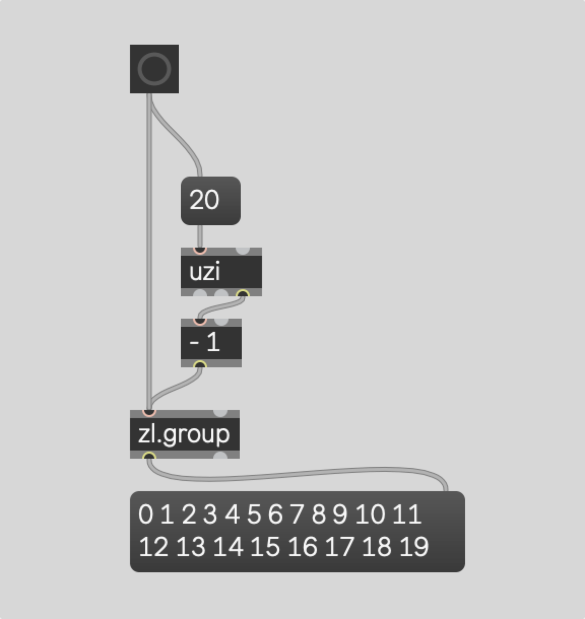
into 20 bands. How could we do that? The uzi object can count from 1 to 20 to represent each
band. If we want to count from 0 to 19 (still 20 bands) then we could do so like this:
We can then map those numbers onto the range of frequencies from 80 hz to 12000 hz using the
scale object.
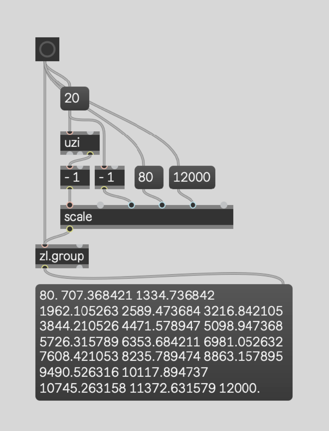
"Great," you say! But look closely... these numbers are not the same as the numbers we used earlier.
They aren't even close. That's because we used a linear mapping. To use the more musical "equal-
octave" logarithmic mapping, we have another trick to employ.
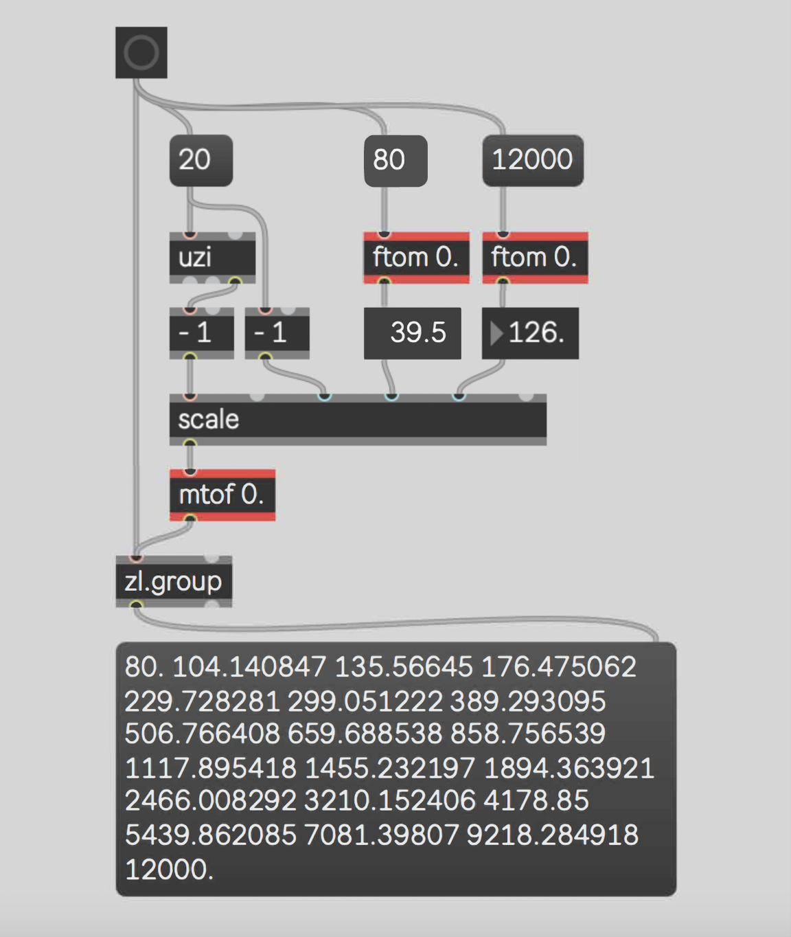
Here we use the ftom object to convert the frequencies into MIDI note numbers. Then we scale
across the MIDI note numbers linearly before converting back to frequencies using the mtof object.
That provides us with the perfect logarithmic curve without needing to think too hard about what
math is going on in there. Note that we need to add the floating-point argument to ensure that the
midi to frequency conversion is accurate and not rounded off.
And Now for the Q
The problem of the "magic" frequencies is solved! Now we just have that magic Q-factor of 7.628.
Where does that come from? How can we hope to calculate it ourselves?
The truth is that we could fudge the Q in many applications. Especially in a vocoder. Whatever the
ideal Q is, you may want to modify it for artistic or aesthetic reasons. The vocoder device in Ableton
Live has a bandwidth (or "BW") parameter that does exactly this.
In other applications, it is more crucial to know the ideal Q-factor and we'd like to understand it here
too. The ideal Q-factor is the Q-factor that results in any two adjacent filters crossing over at -3db.
(If you want to know more about filters and crossovers, I have a series on that too.)
The Q-factor is how steep the filter is. It is based on ratios so that it can apply equally regardless of
the actual frequency you are using in the spectrum. For simplicity, we can use the first 2 frequencies.
When we calculate the ideal Q-factor for those two filters then the same ideal Q-factor will hold for
the rest of the frequencies in the series.
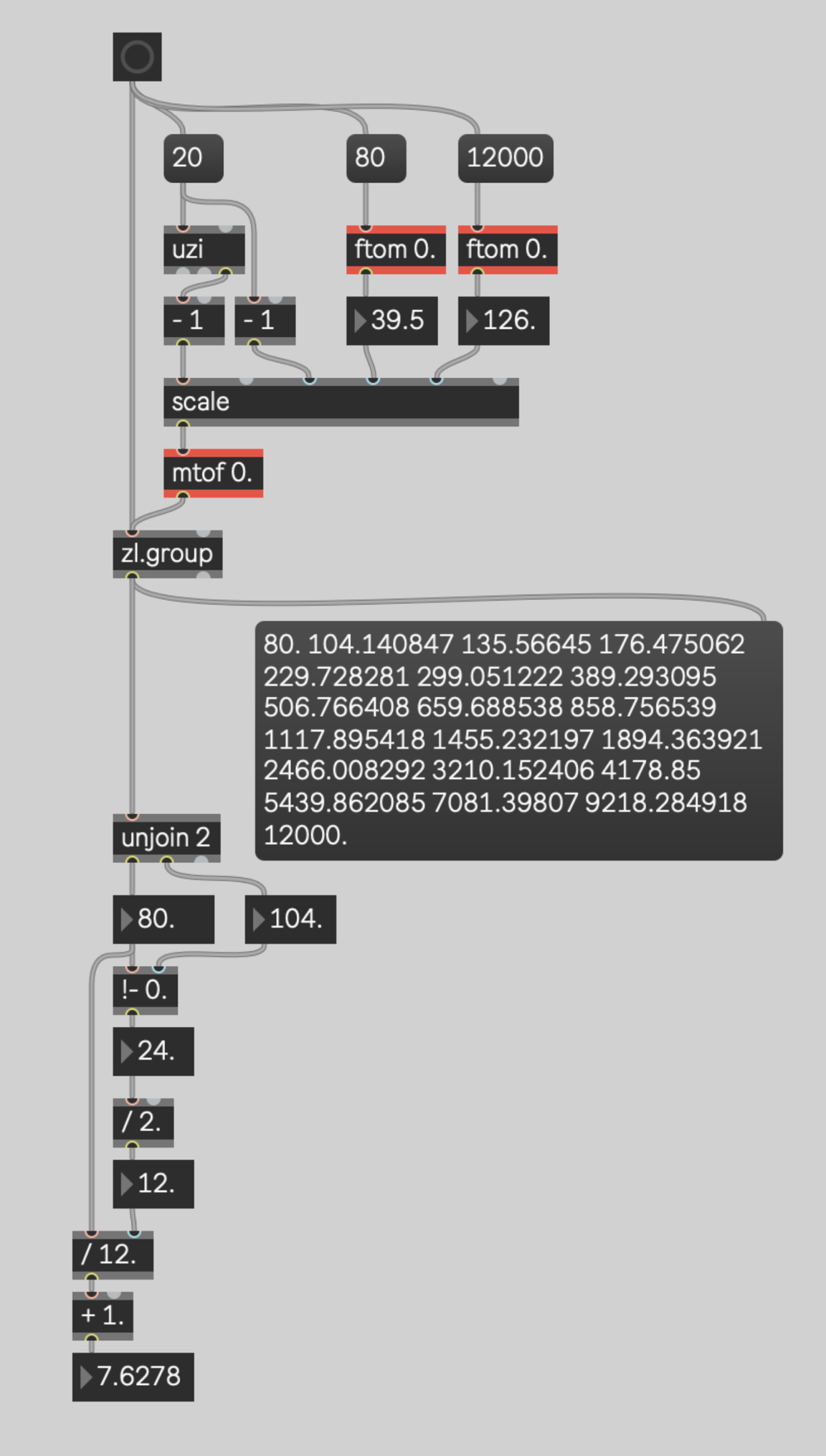
The first two frequencies are 80 hz and 104 hz. The !- object does simple subtraction, it just reverses
the numbers before doing it. So the number box below it shows the result of 104-80 which is 24 hz.
That's the distance between these two filters.
The frequency where we want these two filters to cross over is half way between them. Half way
across this 24 hz chasm, is 12 hz. That means the crossover point is at 92 hz (80+12 or 104-12). So the
bandwidth of this filter is 12 hz and cutoff frequency where it hits -3db is 92hz.
Q-factor, however, is not raw bandwidth. It is a ratio of the bandwidth to the cutoff frequency. So we
divide the cutoff frequency (92hz) by the bandwidth (12hz) and we get our Q-factor of 7.628.
Wrapping it Up
A Real-Time Analyzer is a great tool for visualizing the spectrum of your audio signals in a musically significant way. And it makes an excellent building-block for creating vocoder effects.
The basic concept of the RTA is simple: it's abunch of bandpass filters with audio meters at the end.
The challenging part is figuring out what frequencies to use and how to set the Q-factor. To do that
there is no avoiding some math, but there are ways to intuit the process and think about it in practical
terms. That's what we did here.
The other thing we did was leverage Max 8's MC features. With the tools we employed here, this
patcher can be easily modified to make an RTA of 16, 32, 128 or even 256 bands.
Thanks for following along!
Learn More: See all the articles in this series
by Timothy Place on 2020年8月17日

