Demystifying Digital Filters, Part 1

With this tutorial, we begin part one of a four-part series on digital filter topics. This series will explore a combination of the theory and practice of digital filters, and at the end, we’ll emerge with a better view of what digital filters are, how they work, and which filtering techniques work best for different situations.

This first part of the tutorial series will introduce the key concepts we use when we talk about digital filters:

• systems and signals

• linearity and time invariance

• time and signal domains for filtering

• impulse responses

• convolution versus recursion

What is a filter, anyway?

A filter is a system that produces an output signal based on an input signal. As DSP guru Julius O. Smith III puts it,

Any medium through which the music signal passes, whatever its form, can be regarded as a filter. However, we do not usually think of something as a filter unless it can modify the sound in some way. For example, speaker wire is not considered a filter, but the speaker is (unfortunately). The different vowel sounds in speech are produced primarily by changing the shape of the mouth cavity, which changes the resonances and hence the filtering characteristics of the vocal tract. The tone control circuit in an ordinary car radio is a filter, as are the bass, midrange, and treble boosts in a stereo preamplifier. Graphic equalizers, reverberators, echo devices, phase shifters, and speaker crossover networks are further examples of useful filters in audio. There are also examples of undesirable filtering, such as the uneven reinforcement of certain frequencies in a room with “bad acoustics.” A well-known signal processing wizard is said to have remarked, “When you think about it, everything is a filter.”

When we talk about filters as musicians and Max users, we’re usually referring to systems that modify the frequency content of incoming signals. That’s not the case for all filters — for example, an allpass filter only changes the phase of its inputs rather than its frequency.

As a Max user, you’re already familiar with the idea of a signal as a stream of floating point numbers. A system transforms that signal — you can think of a system as a function or an algorithm. In DSP textbooks, you’ll usually see a diagram that shows a system as a box in between two waveforms, an inlet signal x and an outlet signal y:

Time and frequency

If you’re the user of a filter, it shouldn’t matter much to you what happens to a signal in the time domain–we’re more interested in what happens to the frequencies. When patching or programming, though, you’re more likely to be working in the time domain. With that in mind, it’s a good idea to make sure you know how to travel between the two domains.

To do that, you should know how to use the Fourier transform. Chances are you’ve heard of the FFT (Fast Fourier Transform), which is just what it sounds like – a faster way to do a Fourier transform. If you’re unfamiliar with FFTs and would like a better intuition for them, you can check out this video by Grant Sanderson of 3Blue1Brown and this interactive website by Jack Schaedler. To see more on the practical details as a Max user, head over to the tutorials on the fft~ and ifft~ objects in the Cycling '74 MSP analysis tutorials as well as the Advanced Max FFT video series.

In short, though, the FFT is our ticket to translate between time-based and frequency-based representations of the same signal. Keep this in mind because it will come in handy soon!

Linear Time-Invariant (LTI) systems are our friends

When talking about systems, the properties of linearity and time-invariance are useful in calculations. Fortunately, many real-world systems (and filters) have both of these properties and make the math surrounding them much easier to handle. Specifically, LTI systems allow us to work easily with Fourier analysis, one of the most useful pieces in a DSP toolkit.

For a system to be linear, it has to satisfy two properties:
1. Scaling: The output can only be multiplied by a scalar. This means that you can only multiply the input by a constant value, like a function f(x) = -2x or g(x) = 0.1x or a function like h(x,y) = xy or p(x) = sin(x) does not satisfy this property.

2. Superposition: It should not matter if you add two signals before or after the system. The final result should be the same.

The nice thing about linearity is that it makes it easy to break apart the pieces of an input and do computations separately on those pieces before we bring them back together at the end.

The property of time-invariance might sound confusing at first. How can anything interesting happen to a signal if nothing changes over time? Careful! We’re only making sure that the system (our function or algorithm or black-box, depending on how you like to think about it) doesn’t change over time, not the actual data going through it.

Time-invariance is sometimes called “shift” invariance because it means you can shift where a signal is in time, and it won’t change how the system treats it.

Impulse, frequency, and step responses

When we talk about a filter’s performance, we often look for its “impulse response.” In other words, we want to describe what the output signal of a filter looks like when it’s sent a single, extremely short spike.

The reason an impulse response makes a good “test signal” is that an infinitely short pulse in the time domain is infinitely wide in the spectral domain. This means an impulse contains every possible frequency. (To be technically correct, since our actual impulse has to take up at least one sample, it cannot be infinitely narrow and thus doesn’t actually contain every frequency. However, it is close enough for real-world applications.)

The usefulness of an impulse response becomes clearer when we’re talking about our pal the LTI system. In an LTI system, the impulse response contains all the information about the filter.

From the impulse response, we can take the Fourier transform and find the “frequency response” of the filter, which you may be familiar with.

If you take the integral of an impulse response (or more accurately in the world of digital signals, take a running sum), you can also find the “step response” which shows how the system reacts to sharp transients. You can imagine this as feeding in many 0’s to the system then abruptly switching to all 1’s and seeing what the output looks like. As mentioned earlier, all of these representations contain the same information — they’re just presented differently.

With all of these different representations, we can find out how well our filter does the job we want it to do. For example, if we want a filter that has a steep roll-off, we can check how well it does that by looking at the frequency response. As we learn more about filters, we’ll see that there is no one filter that works for every job, but every job can have a filter tailored for it.

How do you make a digital filter?

You may or may not be surprised to learn that all a filter does is take a weighted average of the buffer of samples moving through it! There are two ways to do this: through convolution or through recursion.

Convolution

The figure below illustrates the process of convolution. We say that the input signal x is convolved by a kernel associated with the system to get the output y. (This kernel is the way we weight the input samples in our weighted average.) The blue boxes are samples whose values are known, and white boxes are samples that aren't known. For each output sample in y, the kernel slides along, lining up its rightmost box with the output sample to calculate. Then, for each matching pair of kernel values and input values, these are multiplied together and then added to get the output value. Once this is complete, the kernel moves to the right another sample and does the calculation again.

Some questions to ponder about this illustration to check your understanding:

1. Where do the values of 41 and 47 come from?

2. What would the next value in the output signal be once we shifted the kernel to the right one sample?

3. Why does the illustration not show the leftmost two output boxes’ values? What information would you need in order to calculate them?

4. The values of the output are much larger than the input’s. What change would you make to the kernel to make the values more similar in size? (Hint: think about percentages.)

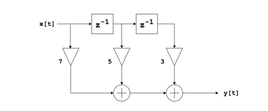
For those coming from Gregory’s recent article on block diagrams and gen~, you may be interested to see the corresponding block diagram for this convolution example:

Now that we’ve looked at one concrete example, let’s try to generalize the convolution algorithm into an equation.

First, start with the additions and multiplications:

To generalize, you can substitute in variables for the values of x:

Then do the same thing for the kernel h’s values:

If you wanted, you could stop here. However, to make this generalized equation more compact, you can use summation notation. Summation notation is useful shorthand for writing out long, repetitive sums. In our example, the sum is short enough to write out, but there are times when you’re adding hundreds of numbers that follow a pattern, and you wouldn’t want to write that out fully. Since long sums show up everywhere in DSP, it’s worthwhile to take a short detour to learn how they work. (If you’re already familiar with summations, feel free to skip down to the final form of our equation.)

Notice that there is a pattern in the equation we just wrote: the first term uses the first value of h (at index 0) and the rightmost value of x (at index t_n), the second term uses the second value of h (at index 1), and the second to rightmost value of x (at index t_n - 1), and so on. If you assign a variable n to the index, then you’ll see in our example that n ranges from 0 to 2. Written in summation notation, this is:

In this notation, the index is defined as n and initialized to 0 and written below the sigma (∑) sign. The end of the range is written above the sigma.

To finish reaching a general equation for convolution, let’s write what the sum would look like if the kernel size was also a variable. Let’s call it N. Since we’re describing any t, not just the specific t_n of our example, let’s drop the subscript, too.

Because convolution is such a useful operation, you can also use the “star” operator to write this equation in an even shorter way.

Note: There is a difference between seeing a star between two functions and two variables or values. In the first case, that means convolution, but in the second case, it means multiplication. Confusing, yes, but it’s what mathematicians have stuck with. Usually you won’t see the star being used to mean multiplication in DSP papers/books/articles/etc., though, so the possible confusion isn’t as likely as you might fear.

The reason for looking at these kinds of generalized equations is because it’s an easy way to describe filters in a mathematical way without drawing any diagrams. These kinds of equations describing filters are called difference equations. (You’ll see why they’re called “difference” equations rather than “summation equations” later on in this series when we talk about IIR filters.)

Impulse responses of convolution filters

With notation out of the way, let’s return to the filter we’ve made and illustrated. To see how the filter performs, remember that impulse responses are the best way to learn about a system. Let’s calculate a few samples of the impulse response by hand.

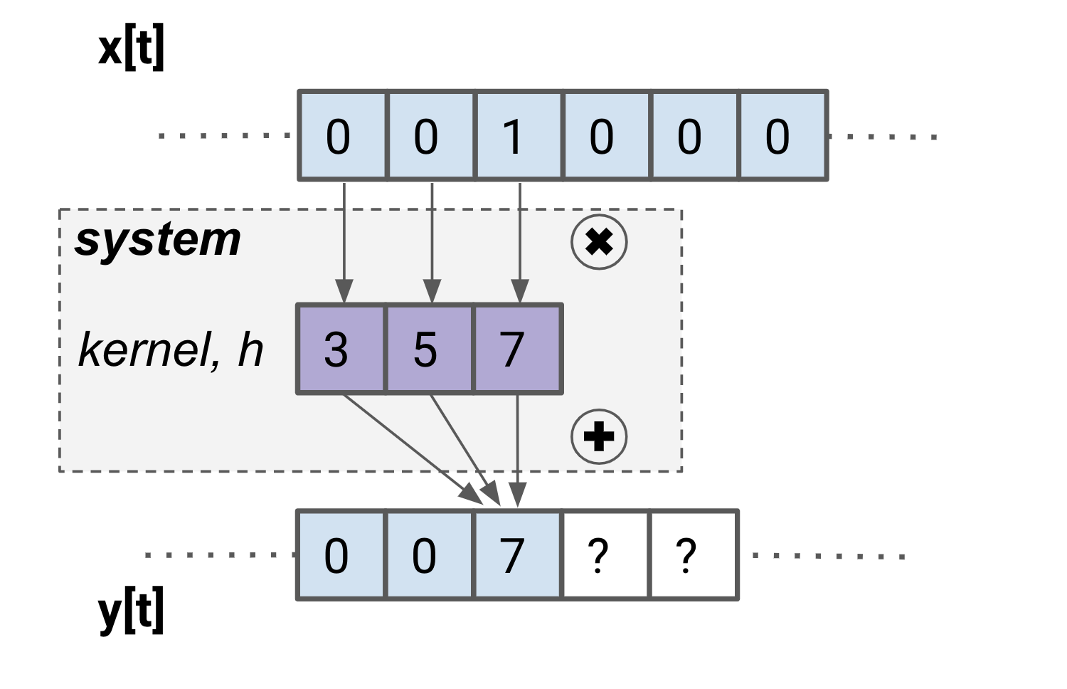
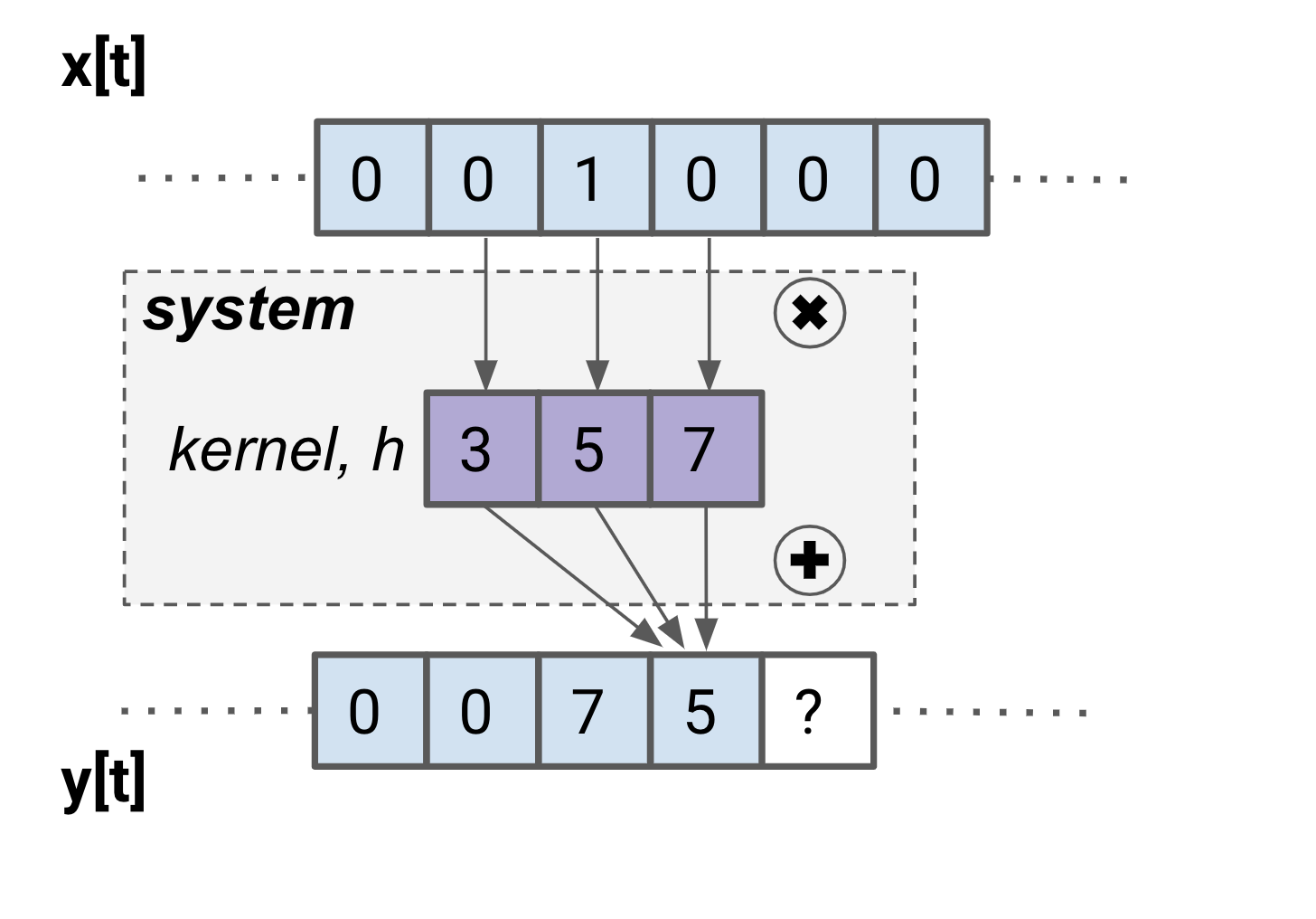
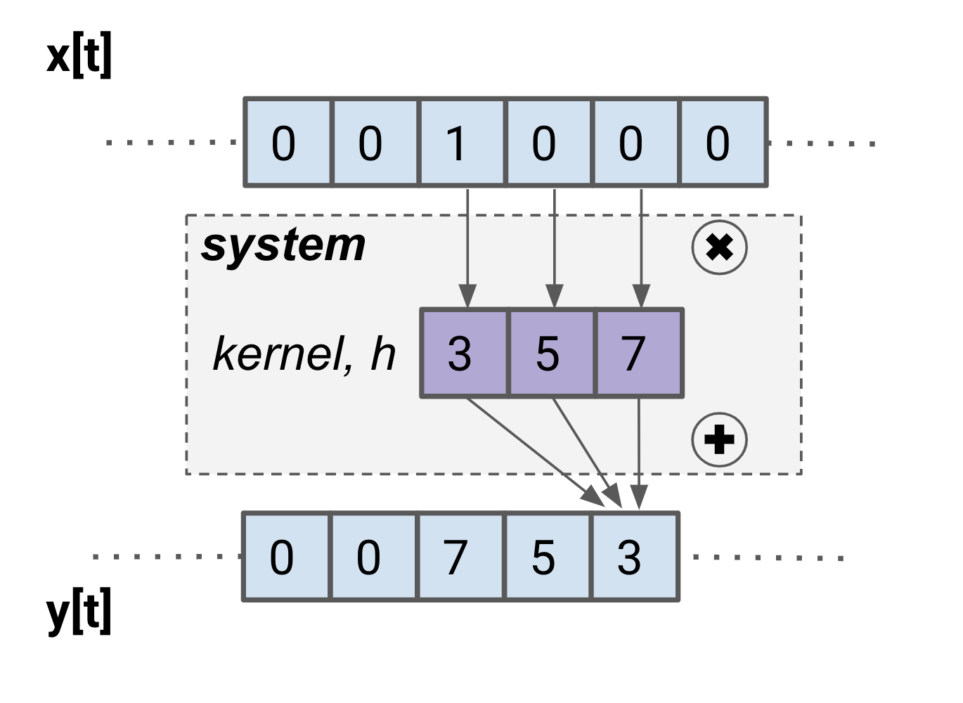
From this exercise, you can see that by convolving an impulse with the kernel, you get a backwards version of the kernel as the output! You may recognize that this isn’t just luck – for any LTI system, the kernel comes directly from the impulse response.

Armed with the knowledge you’ve gained so far, you can start to think about the ways we can design a filter that uses convolution. In our first example, we tried playing around with values of the kernel and looked at the outputs we could get. Our other option is to go in the other direction – start from the output signal we want and compute the kernel.

To do that, remember that you can use the Fourier transform to find the frequency response from the impulse response. Often you know the frequency response you want, so it should be possible to find the filter kernel from there. The steps are as follows:

1. Create the desired frequency response curve.

2. Compute the impulse response using the FFT on the frequency response.

3. Use the impulse response as a convolution kernel.

This kind of filter (one that uses convolution) is called a Finite Impulse Response (FIR) filter. The easy way to remember this is that an impulse response has to be a finite length to do convolution with it. The corollary of this is often used in textbook definitions of FIR filters–impulse responses always decay to zero in finite time when using FIR filters.

We will go more in depth on FIR filters in Part 2 of this series, but until then, let’s take a brief look at the other kind of filters, recursive filters.

Recursion

Readers with a sharp eye may have noticed something about the convolution algorithm and the FIR block diagram – the output only uses the input samples. This means that we’re only using feedforward loops, never feedback.

If you were to use both feedback and feedforward, you would be making a recursive filter. Notice that for recursive filters, we use the terms “feedback coefficients” and “feedforward coefficients” instead of “kernel.”

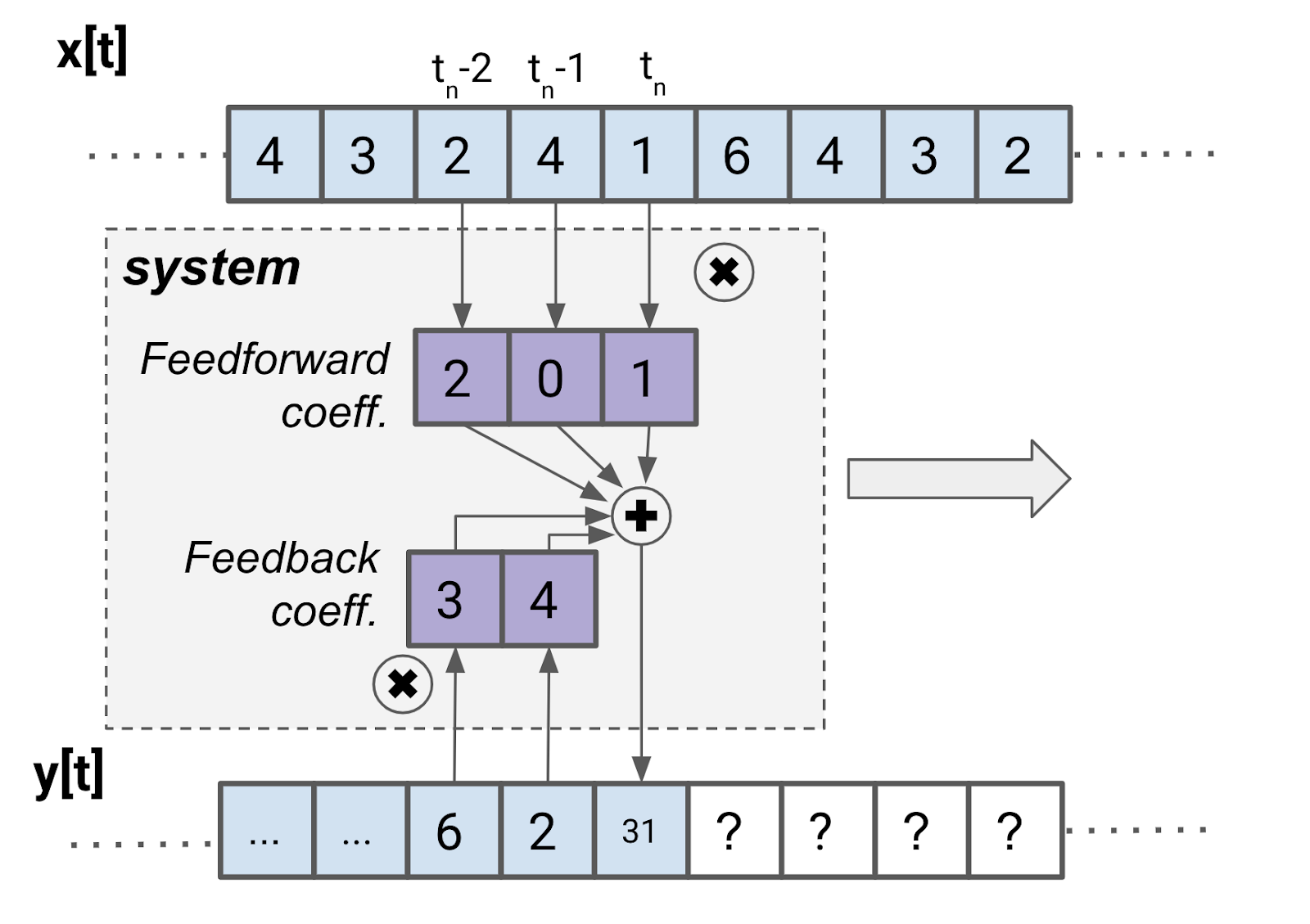
You’ve likely seen block diagrams for recursive filters before if you’ve looked at biquad filters.

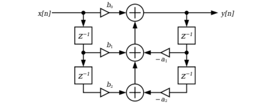
Once feedback loops come into play, there’s no guarantee that the impulse response will decay to zero in finite time any longer. (This isn’t always the case, though. There are some situations where recursion can be used to create FIR filters, but that’s a topic for another time.) These filters with infinitely decaying impulse responses are called Infinite Impulse Response (IIR) filters. When doing your own research, you may also hear them called recursive or feedback filters. We will learn much more about IIR designs in a later section of this series.

What’s next?

We’ve covered a lot in this tutorial, and there is plenty of ground remaining for more exploration! Up next, we’ll take a deeper look at FIR filters and discuss when they’re best suited for your filtering needs.

References

• The Scientist and Engineer's Guide to Digital Signal Processing by Steven W. Smith

• Introduction to Digital Filters with Audio Applications by Julius O. Smith III

• Digital Biquad Filters, Wikipedia

• MIT Open Course Ware 6.007 Signals and Systems

Learn More: See all the articles in this series