Advanced Max: An Inquiry into Max’s Slide Objects

Introduction

Max is graced with many filters, taking on many guises - some of which we don’t even think of as filters in the classical sense. The help patcher for the slide object says that it “smooths values logarithmically” - indeed, it does. It is, together with the slide∼ and jit.slide objects, a lowpass filter.

In the process of exploring the algorithm used in these objects, we'll see how they relate to canonical filters with which you may be more familiar. Along the way, we'll step through the mathematical procedures, one step at a time. In the interest of being thorough, I'll try to minimize assumptions and introduce even basic mathematics explicitly.

Note: Readers desiring a quick brush-up to help with following the mathematical expressions are urged to do so before proceeding. Khan Academy is a tremendous resource for reviewing (or learning) algebra by starting with the short videos. If you want a quicker jump-start (or something more basic than algebra) check out the the pre-algebra videos here.

Conventions and Presuppositions

The following descriptions use the standard filter nomenclature where:

n references the current sample location

n−1 references the previous sample location (meaning delay of 1 sample), etc.

x(n) is the current input.

y(n) is the current output.

So, x(n−1) is the immediately previous (or delayed) input, and y(n−1) is the immediately previous (delayed) output, etc.

a₀ is a coefficient to be applied to the FIR side of a canonical filter. As examples, a₀ is the coefficient applied to x(n−0), a₁ is applied to x(n−1), etc.

Likewise, b₁ is a coefficient to be applied to the IIR side of a canonical filter - that is, b₁ is the coefficient applied to y(n−1), b₂ is applied to y(n−2), and so on. There generally is no b₀ because the current output is unknown at the time the calculation is being performed.

The constant fs is the sampling frequency (also known as the sample rate).

Background and Applications

There many ways to smooth a stream of numbers. Perhaps the simplest is to average them. Classic averaging is a lowpass filter with a “finite impulse response”. This is discussed in videos and provided in complementary gen∼ patchers published by Cycling ’74.

Averaging has a number of benefits, including linear phase response and the straight-forwardness of the calculation. The slide objects are nowhere near as easy to describe as the average∼ object, but they are far faster to compute.

All three of the slide objects - slide, slide∼, and jit.slide objects calculate their output identically, so the formula given in the reference pages for each of the objects is the same. For the purposes of this discussion, I'll focus on the slide∼ object for processing audio, because it simplifies the relationship to real time.

Besides generalized smoothing for parameter control, a good use for this type of filter is to slow down the decay part in

audio rate envelope following. Algorithms akin to this are often used in compressors/limiters as well as visualizers for music playback software.

slide∼

The slide∼ object implements a “logarithmic” filter with a slide parameter to smooth out discontinuities in an input signal, such as for performing envelope following. The slide∼ object actually contains two filters: one filter for changes to the input that increase in value (‘slideup’) and one filter for changes to the input that decrease in value (‘slidedown’). Often these are set to the same value, which simplifies some of our expressions, so for this discussion I'll take this to be the case and simply use the term slide for both up and down.

Given a slide value of 1, the output will always equal the input. Given a slide value of 10, the output will only change 1/10th as quickly as the input - this description of the slide∼ object’s behavior can be found in the object’s help patcher and reference page. Putting this in terms of time is complicated, or even exactly in terms of an average of N samples, since that wouldn’t be precise either. Nor is it exactly easy to describe in terms of weighting (the current incoming value is weighted by 1/N and then you have an exponentially decaying curve as you look towards samples from the past).

Mathematically, the filter can be expressed with the equation

slide

This equation expresses the filter in terms that relate to the original description of the object. However, this equation also obscures a number of characteristics of this filter, making it difficult to relate to other filters in Max. If we rewrite the equation in the terms of a standard difference equation we can glean some insights into the operation of the slide∼ object. We start with the equation as originally expressed

Letting a₀ = 1/slide, we can continue to rewrite the equation as

Equation 2 re-expresses equation 1 in terms that of the general difference equation. One immediate use of this is that we can plug the numbers into Max’s biquad∼ object to perform the same filtering, or use the filtergraph∼ object to plot the frequency and phase response. With the equation in this form, we can also see that there are two coefficients: one for the gain of the filter’s input and one to control the gain of a first-order pole, meaning that all we have is a simple one-pole filter. So, we could also plug the coefficient into the onepole∼ filter object to do the same thing.

Frequency Response

Now that we know that the slide∼ object is simply a one-pole filter, we can calculate its frequency response for any given value of the slide parameter. Remember that we have two coefficients derived from the slide value.

The onepole∼ object uses these same coefficients, but typically calculates from a desired cutoff frequency in hertz fʜᴢ. The first step is converting fʜᴢ, which depends upon the sample rate fs, into a sample rate independent form expressed in radians fʀᴀᴅ.

One potential confusion regarding radians is the fact that, in Max, some objects have a ‘radian’ mode which is expressed in something resembling radians but does not map to frequency with a linear relationship. Examples include onepole∼ and svf∼. It is unfortunate that this special mode was named ‘radian’ since it is misleading and confusing. Their use should be considered deprecated.

As an example, we can let fʜᴢ = 1000 and fs = 44100. Then

Given the frequency in radians, we can now calculate the coefficients

To simplify things, let’s combine the conversion into radians into the coefficient calculation

The relationship between a₀ and b₁ is the same for the onepole∼ coefficients as it is for the slide∼ coefficients, reinforcing the fact that these are really the same filter. We now have enough information to relate onepole∼’s fʜᴢ parameter to slide∼’s slide parameter through a₀.

To solve for slide in terms of hertz we can flip the fractions, resulting in

or to solve for the cutoff frequency in terms of slide

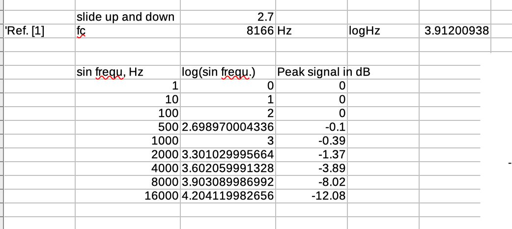
See the table below for some example values to see how the slide parameter relates to the cutoff frequency when using a sample rate of fs = 44100.

Further Exploration

Smoothing algorithms analogous to slide in other environments include Faust. Further exploration of this class of filter is left as an exercise to the reader. If you're interested in pursuing this topic, the Moving Average article on Wikipedia serves as a reasonable point of departure.