Demystifying Digital Filters, Part 3
Part three of this series will lay the conceptual groundwork required for designing and analyzing IIR filters, the counterpart of FIR filters. This article will cover:
Filter kernels vs. filter coefficients
Difference equations
Transfer functions
Filter order
Poles, zeros, and stability analysis
IIR versus FIR
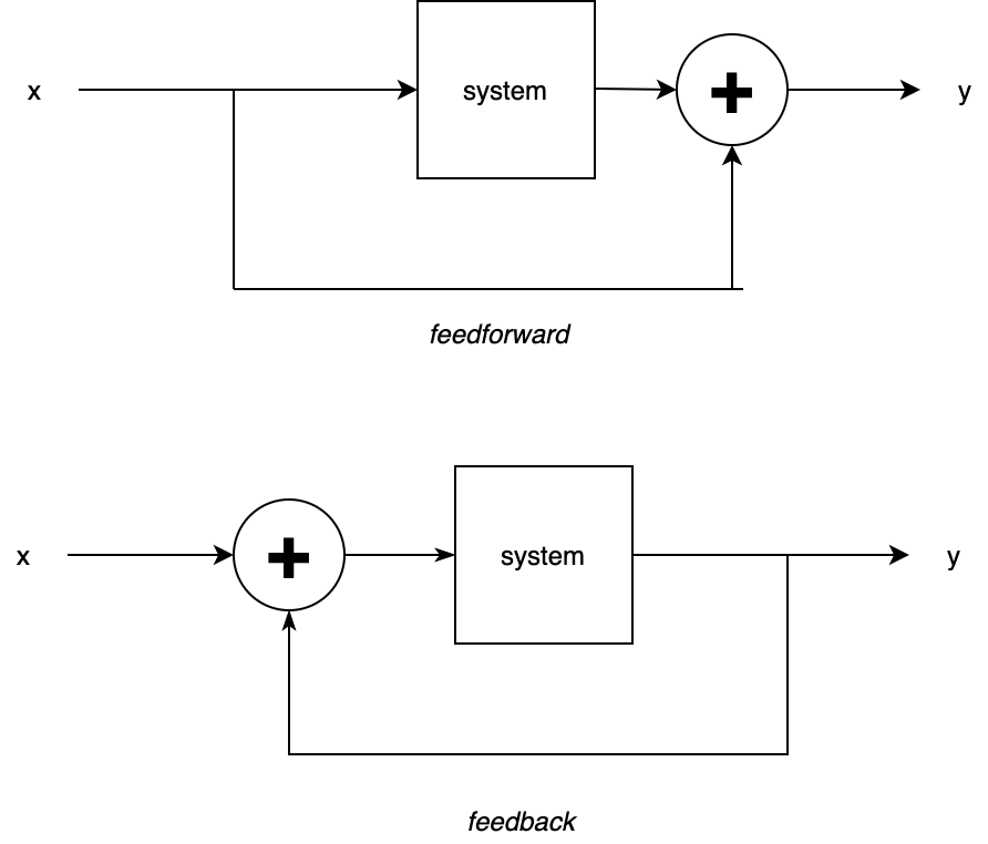
Recall from part one that FIR and IIR filters are quite similar in implementation — they are simply weighted average machines. The difference is that FIR filters require only feedforward loops (relying only on input samples) whereas IIR filters use both feedforward and feedback loops (relying both on input and output samples).
Why might you use an IIR implementation over an FIR one?
Advantages:
Lower latency, fewer coefficients needed for the same specifications as an FIR filter
Easier to model analog filters
Easier to tweak parameters on the fly
Disadvantages:
Less numerically stable (feedback loops can cause unbounded growth)
Nonlinear phase response
Despite their disadvantages, IIR filters are a common choice because they are less memory-intensive and many applications do not require linear phase responses.
Kernels, coefficients, and the difference equation
Remember that filters are just weighted average machines, and the work of filter design is to define the weights used in that machine. In FIR filters, we referred to these weights as the filter kernel, but they can also be called filter coefficients. Since the term kernel is associated with convolution, IIR filters — which don’t use convolution — stick to calling them coefficients.
The word “coefficient” makes sense when you think about the relationship they have with the generalized equation for the output y of an FIR filter:

Notice that once you expand out the summation, the kernel values (h[n]) act as coefficients for each of the terms from input signal x. For example, a kernel with three values expands to:

Recall that another word for the generalized formula for computing outputs of a filter is a difference equation. You know what difference equations look like for FIR filters, but what about IIR filters?
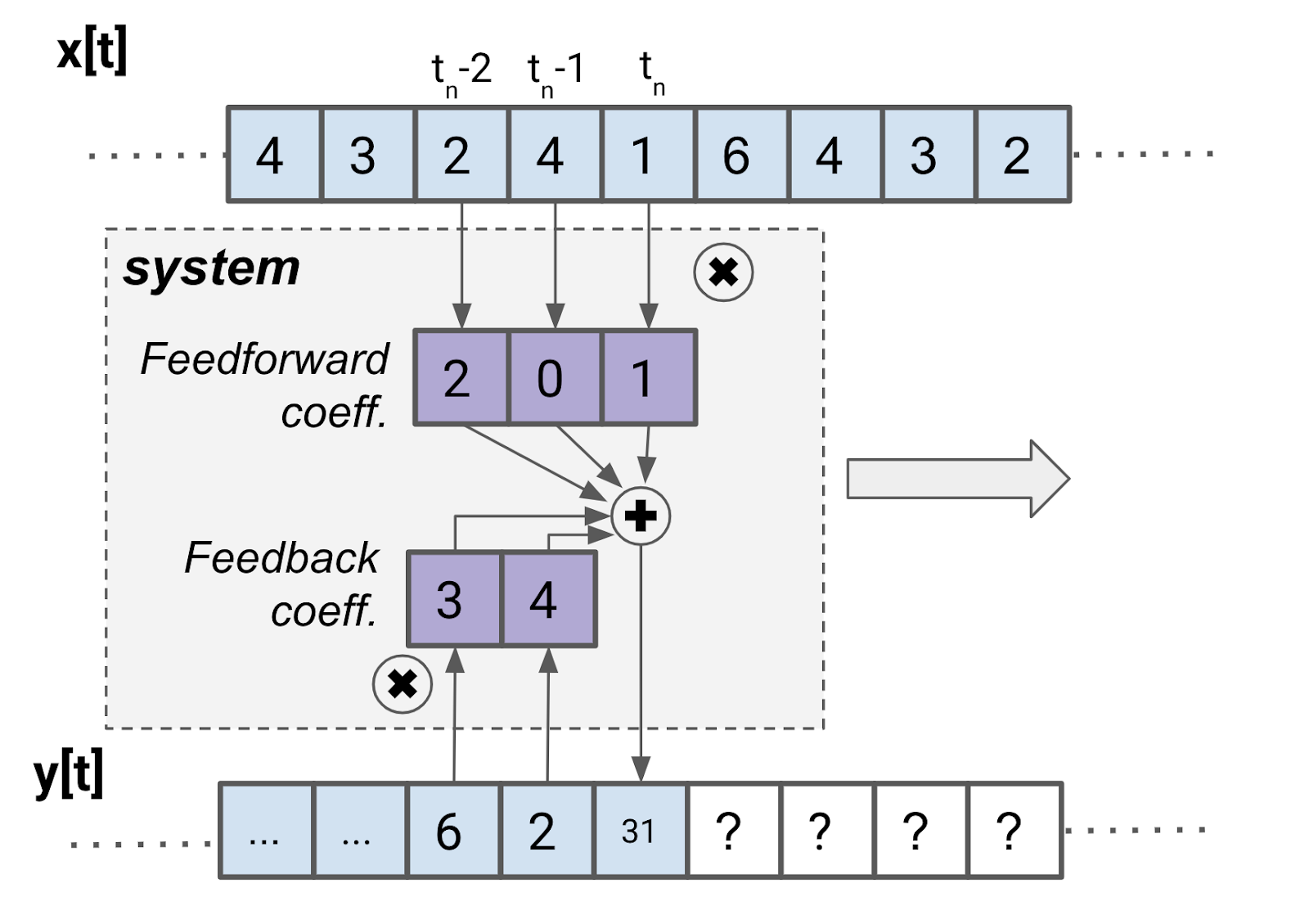
Let’s try an example:
The summing and multiplying to find y[t_n] is:

With IIR filters, we distinguish between feedback and feedforward coefficients. By convention, feedback coefficients, given the letter a, are written with negative signs in front. Feedforward coefficients are given the letter b. The subscript of the coefficient is associated with the delay (in units of samples).

Replacing values with variables gives:

Gathering up terms into sums:

Finally, for M feedforward coefficients and N feedback coefficients, you can write more generally:

Seeing the prominent subtraction of the two summations should now explain why the equation is called a “difference” equation!
Another new representation
So far we’ve discussed a number of interrelated ways to represent a given filter. If you know any one of the following, you can compute any of the others, assuming the filter is LTI:
Impulse response
Frequency response
Step response
Filter kernels/filter coefficients
Difference equation
Besides the representations you’ve learned so far, there is yet another one called the transfer function. The transfer function is the key to analyzing filter properties you may have heard of before, including:
Filter order
Poles and zeros of a filter
Filter stability
Why wait until now to look at transfer functions? Well, since FIR filters don’t run into the same stability problems as IIR filters, transfer functions are much more interesting to analyze for IIR filters. Furthermore, poles and zeros are used in IIR design and not so much in FIR design.
Before discussing these filter properties, let’s first look at how you can find the transfer function from the difference equation using a very close relative of the Fourier transform — the Z-transform.
The Z-transform
Remember that the Fourier transform is a way to “translate” between a frequency and time representation of a signal. To do this, the Fourier transform uses sinusoids as a building block by mixing together sine waves of different frequencies and amplitudes to represent any other signal. In the world of math, this “mixing” is called a linear combination and sine functions are considered the basis. What if, instead of sine waves, you could use another kind of function as a basis?
The idea of the Z-transform is to use a complex exponential function, represented by the letter “z”.

In this equation, the A represents some amplitude, i is the imaginary number, and ϕ (phi) is an angle.
Complex exponentials may be intimidating at first, but they’re incredibly practical for two reasons:
It’s often easier to do operations on exponential functions compared to trigonometric ones.
Complex numbers wrap up two pieces of information into one. (You could think of complex numbers as being two-dimensional versus a one-dimensional integer.)
The Z-transform is defined as follows:

(Note for completeness’ sake: There are two similar forms of the Z-transform, the bilateral transform and the unilateral transform. The form above is the bilateral one, but the differences in the two forms won’t make a difference for the scope of our discussion.)
The left hand side of the equation is saying that the Z-transform operates on a signal x that is indexed by integers n.
On the right hand side, the transform is defined as a sum over values of n from negative to positive infinity. This just means that every value of x is considered; if you had 12 samples in x, for example, you’d have a sum of 12 terms. Each of the terms in the sum is a value of input x (at index n) multiplied by the complex exponential z raised to the negative n power.
From this you can see what makes the Z-transform so similar to the Fourier transform — it represents an input signal as a sum of many sinusoids (only this time, those sinusoids are wrapped up in a complex exponential function). In fact, if you set z = e^{i * ϕ} in the Z-transform, you would get back the definition of the complex discrete Fourier transform. The difference between the two is just that pesky amplitude A in the Z-transform!
What does the Z-transform of a simple example signal look like? Let’s use a signal x that is two samples long. (Note the new shorthand for the Z-transform, too. A capital letter with an argument of z represents the Z-transform.)

You can drop away z^0 since that just equals 1, and then you’ll find:

Another note: Now you see why block diagrams show a single sample delay with z^(-1) notation! This is related to what is known as either the shift-invariance or time-delay property of Z-transforms, which you can learn more about (along with other properties of the Z-transform) here.
If you ever want to avoid doing the work of performing a Z-transform by hand, you can try using Wolfram Alpha’s Z-transform calculator.
Finding the transfer function
The basic form of a transfer function H(z) is a ratio between the Z-transform of an output signal y versus an input signal x.

To see how you might find a real-world transfer function given a difference equation, let’s walk through an example of an IIR filter’s difference equation.

First, gather the output signal terms on the left and the input signal terms on the right.

Next, write each term as its Z-transform.

Do a little rearranging, taking advantage of the linearity property of the Z-transform so that X(z) and Y(z) can be factored out.

One more step...

Congratulations! Meet your very first transfer function.
Filter order
Transfer functions are often represented in a factored polynomial form. In other words, the “shape” of a factored transfer function will look something like:

There will be some constant gain factor in front and the numerator and denominator will be a bunch of terms multiplied together where each term is 1 minus some factor times z^(-1).
Your first transfer function, for instance, slightly rearranged to be in factored form is:

In this case, the numerator and denominator only have one term, but there is no limit to how many terms you can be. This brings us to the concept of order — the filter's order is the order of the transfer function. To find the transfer function order, find the degree of the numerator and the degree of the denominator (by counting the number of z^(-1) terms are in the factored form). The maximum of those degrees gives the transfer function order. If, for instance, there were three terms in the numerator and four terms in the denominator, the transfer function would be “fourth-order” since max(3, 4) is 4.
In general, a higher order means a better quality filter (with a steeper slope). At the same time, a higher order means more computational effort is needed. Can you think of why longer delay lines are needed for higher order? (Hint: Think about what the difference equation would look like as more z^(-1) terms are added. How many previous samples will the calculation need?)
With the filterdesign, filterdetail, and plot~ objects in Max, you can play around to see the effect of filter order on the corresponding frequency response.
Poles, zeros, and stability
Let’s make up a new transfer function that is higher-order and a bit more exciting to analyze.

First question: what if one of the terms in the top was zero? For instance, what if z was 0.4, 0.3, -0.15, or 0.35? In other words, what if z was a root of the numerator polynomial? The term in parentheses would become (1 - 1), or zero, making the entire transfer function equal zero for that point. These values would be the so-called zeros of the transfer function. These are associated with the feedforward filter elements. Can you convince yourself of this by revisiting the first transfer function derivation?
Similarly, what if one of the terms on the bottom was zero? If z was one of the roots, 0.75 or 0.25, the bottom would equal zero, making H(z) undefined. These are the poles of the transfer function, and they are associated with the feedback part of the filter.
These poles and zeros are often illustrated on a pole-zero plot. Remember that z is an imaginary number, so plotting it occurs on the z-plane (the complex plane) where the horizontal axis is the real part and the vertical axis is the imaginary part. Note that in our example, all of the poles and zeros have imaginary parts that are zero, but this doesn’t have to be the case (and it often won’t be).
To explore the pole-zero plot, the zplane~ object in Max is a useful tool. You can manipulate the poles (shown as x’s) and zeros (shown as o’s), and it will output filter coefficients that filtergraph will understand and plot on a frequency response graph.
As you play with zplane~, you will notice that the poles and zeros mirror across the horizontal axis. This is explained by the complex conjugate root theorem. The theorem basically says that for any root of a complex-valued function a + bi, there will be another root a - bi.
Finally, you’ll notice that pole-zero plots usually show the unit circle. Why? In short, it’s a way to indicate where a filter will be stable. If any poles lie outside of the unit circle, the filter will become unstable, causing any input to blow up to infinity at the output. (For a mathematical proof of the fact, check out this resource from Julius O. Smith III.) This explains why FIR filters are always stable — they can only have poles at the origin.
Conceptual map
As you reflect on the concepts introduced so far in this series, the following illustration may be a helpful visualization of the relationships between them.
Up next
In Part four, you will build on the concepts introduced in this article by learning about design and implementation of IIR filters.
References
Theory and Application of Digital Signal Processing by Lawrence R. Rabiner and Bernard Gold
Introduction to Digital Filters with Audio Applications by Julius O. Smith III
Learn More: See all the articles in this series
by Isabel Kaspriskie on March 16, 2021


