Gen Tutorial 2a: The Joy of Swiz
Welcome to the second in a series of “drive-by” tutorials – quick introductions to the world of Max Gen objects. While the Gen world is deep and subtle and you may eventually find yourself thinking about things like polar coordinate conversion, dot products, and other bits of arcana, you can still do some rewarding things armed with a few basic concepts and the will to play.
All tutorials in this series: Part 1, gen~: The Garden of Earthly Delays, Part 2a: The Joy of Swiz, Part 2b: Adventures in Vectorland
Reading This Tutorial (And The Next One)
You’ll notice that this is Gen Tutorial 2a, and that it showed up alongside its fraternal twin Gen Tutorial 2b on the very same day. They’re closely related, but very different. In this first tutorial, we’re going to introduce some basic concepts about working in the Jitter Gen environment in ways that closely resemble your experience in the Max world.
Our suggestion is that you go through Tutorial 2a, learn about swizzling, play around with the patches and then dive right back into Tutorial 2b. The second part of the tutorial takes the concepts you learned and the patches we showed you and rewrites them with more efficiency by making use of the vector nature of the Jitter Gen environment.
The Lay of the Land
While the programming you do inside of any Gen object looks and feels like regular Max patching (connecting object boxes together with patch cords in ways that show you the flow of data), there are some important differences that are useful to know when you begin.
The Jitter Gen objects are no exception. They’re even a little different than the gen~ object you use for audio processing, in fact.
The things that happen inside of a Gen object are synchronous – there are no triggers and there’s no notion about the order in which things happen. In the Jitter world, the basic unit of data is a vector, which we’ll describe in greater detail in a minute. For now, think of this vector as a way to collectively describe a group of single pixels rather than a frame of video. Actually, it’s more correct to think of it as though you’re performing the same operation on every single individual pixel (unit of data) in the entire matrix at once.
To provide user input used for calculations and transformations inside a Jitter Gen object, we use the Gen param operator.
Most of the Jitter family of Gen objects only allow you to have a single outlet for your objects – you can have as many single matrix inputs as you’d like (each of which represents a single matrix), but only one output. The jit.gen object is the only exception to this rule.
There’s no way to retain the value of the pixel you’re working on from one operation to the next - if you’re familiar with the gen~ object, there’s no such thing as a history operator for Jitter Gen objects that you’d use for interpolation or filtering or delays (Don’t worry – there are ways to do what you’d use a history object for, which we’ll talk about in another tutorial).
Meet the family
The first thing you’ll notice about using Gen in the Jitter world is that there are three objects instead of one. Here’s how they differ:
The jit.pix and jit.gl.pix objects are made for standard Jitter 2d image processing. They work with input matrices with 1 to 4 planes, and treat incoming data like image data. The jit.gl.pix differs from the jit.pix object in that does all its work on the GPU (Graphics Processing Unit) instead of your CPU.
The jit.gen object is a general matrix processing object that works with any type of data that a matrix can contain (e.g. OpenGL).
In (both halves of) this tutorial, we’re going to be working with the jit.pix object.
Maps Make the Journey More Interesting
As we’ve said before, when you work with Jitter Gen objects, it’s easiest to think of it as performing the same operation on every single individual pixel (unit of data) in the entire matrix at once.
At a very low level, that’s how things like the jit.op or jit.expr objects work – a single operation is performed on each and every individual cell of the matrix or some part of the matrix, and the result of the calculations inside of your Jitter Gen object pops out the outlet of the object as a single matrix.
Let’s start with a really simple Jitter Gen patch. I’m a big fan of color mapping as a way to generate visual variety, so I'm going to start with a simple Gen patch that uses a cosine function to do some color remapping.
The inside of the jit.pix patch is much simpler than you might think from watching its output, but that’s because the relatively straightforward calculations on the inside of the patch are being applied to each and every pixel in the image (actually, the calculations are being performed on each and every pixel in the alpha, red, green, and blue planes).

Note: If you’re accustomed to only working with color in Jitter as char data in the range of 0 – 255, you might be wondering where the color processing is. Jitter actually has an additional way of specifying and working with color values - floating point values in the range of 0 - 1.0. In genland, colors are always specified using floating-point numbers.
Each input pixel is multiplied by an input value and then used as the input to a cosine function. Since we know that cosine functions output values in the range from -1.0 to 1.0, we’ll multiply the cosine function’s output by 0.5 and then add 0.5 to produce values in the 0. – 1.0 range that we expect for colors. The result is quick and easy color remapping - I particularly like the kind of results you get from using large values for the amp parameter.
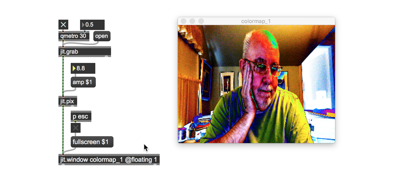
Of course, we could replace the cos operator with any other kind of calculation we could think of (a sin operator would also work well, since its outputs fall into the same range as that of the cos operator), as long as we know in advance what the maximum and minimum values for the output range is so that we can coerce them into the 0. – 1.0 range.
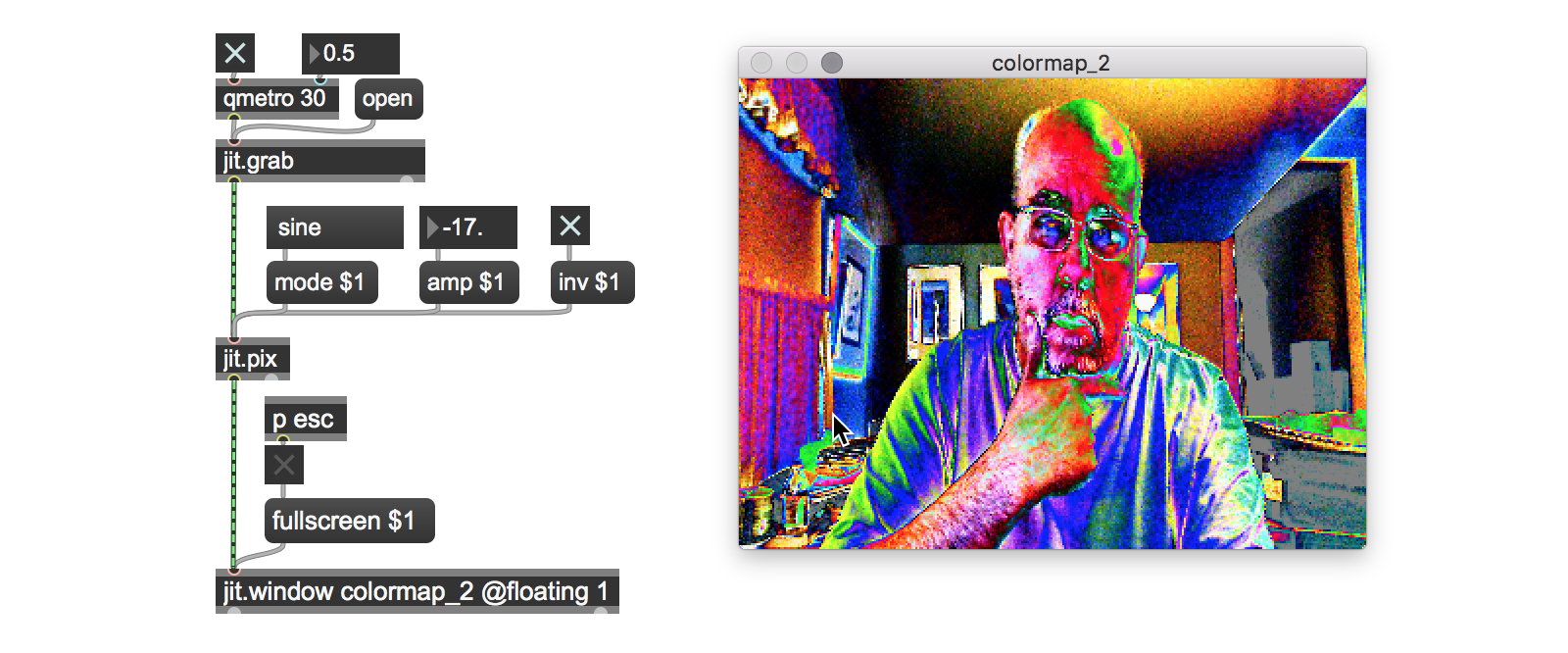
In fact, the tutorial patch colormap_2a does precisely that. The patch not only adds the ability to pass the output unchanged, to select from either cosine or sine mappings, but also lets you choose to pass the data unchanged or invert its output for the passed or processed images. Here’s what the patch inside our jit.pix object looks like now:
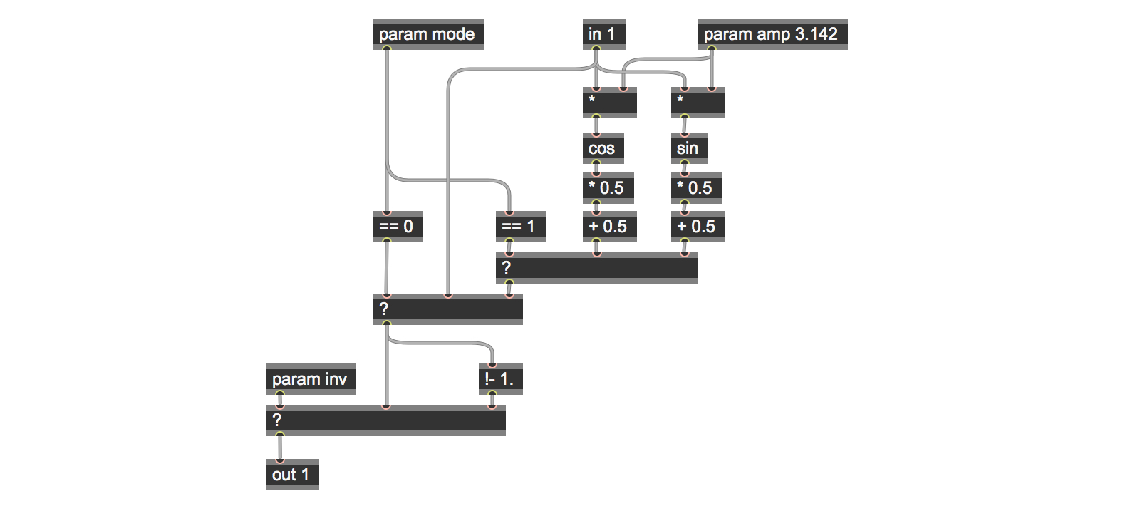
We handle the mapping and inversion in our patch using the Gen ? operator for the logic that allows us to choose whether to pass or process the color values (based on the mode parameter), and to choose whether or not to invert the output (based on the inv parameter).
Each ? operator takes the result of a test in its left inlet. If the input is positive (1), then the input to the second inlet of the object is passed to the outlet. If not, the right inlet’s input is passed.
The parameter values we send to our patch to choose the processing mode are set using the mode parameter – 0 to pass the unprocessed values, 1 to use cosine processing, and 2 for sine function processing. In the same way, the inv parameter is used to invert the color values for the output. Since all of our color values are in the range 0. – 1.0, then we can use the humble !- operator with an argument of 1.0 to do the inversion for us. These minor additions to our patch greatly increase the variety of outputs.
Note: If you’re wondering why we don’t use a selector object inside of our jit.pix object to select the pass/cosine/sine modes instead of two ? operators, then you must be someone who’s gone through my first gen~ tutorial. At present, the Jitter Gen objects don’t have a selector operator.
Fo’ Swizzle
For our next tutorial patch, we’re going to look at what the Jitter Gen objects do on a lower level. As I’ve said, you can use jit.pix to specify arbitrarily complex operations to be performed on each cell – in this case it’s similar to what the jit.expr objects do.
When you work with collections of single pixels in jit.pix, what kind of data can you actually work with? If you’re familiar with how video data in Jitter is represented in matrix form, it’s not hard to guess:
You can fetch data about each individual plane of the matrix for each cell (in video terms, that means the values for the red, green, blue, and alpha channels of the image. If you were working with OpenGL data, it would involve accessing each of the twelve attributes for each vertex associated with an OpenGL object.
You can fetch data about the location of each cell in the matrix (x and y coordinates)
You can fetch data from any other individual pixel in the matrix by specifying its location.
You can write data to the current pixel.
The technical computer graphics way to say this is that incoming pixel data is presented as a grouping of numbers that represent the information about the current pixel called a vector. In Max terminology, the Jitter family of Max objects take matrices (which are, after all, as a grouping of numbers that represent the information about images/OpenGL, etc.) as inputs, process them as vectors of data, and output standard Jitter matrices.
For our next patch, we’re going to look working at with the color values associated with individual pixels, and combine that with some simple Gen logic to create an expanded variation of our previous patch.
I’d like to introduce you to two complementary Jitter Gen operators that will become your friends: swiz and vec. When starting out working with Jitter Gen objects, I found it easiest to think of swiz as the equivalent of unpack, and vec as the equivalent of pack.
Note: Although the names for the operators may not seem obvious, these two terms for operations that let you access individual parts of a vector and recombine are in wide use in the computer graphics world.
The swiz (short for “swizzle”) operator lets you fetch a portion of a vector by specifying it by name. You can fetch individual items or only a single item based on the arguments you give the swiz operator.
The vec (short for “vector”) operator concatenates and outputs a single vector from its component parts for output.
When you work with images in Jitter Gen objects, the names you use when pulling an input vector apart to work with individual color values are nice and easy to remember: r (red), g (green), b (blue), and a (alpha channel).
In our next patch, we’re going to take the cosine trick from our last patch, and add a twist: you’ll be able to operate independently on each of the RGB values.
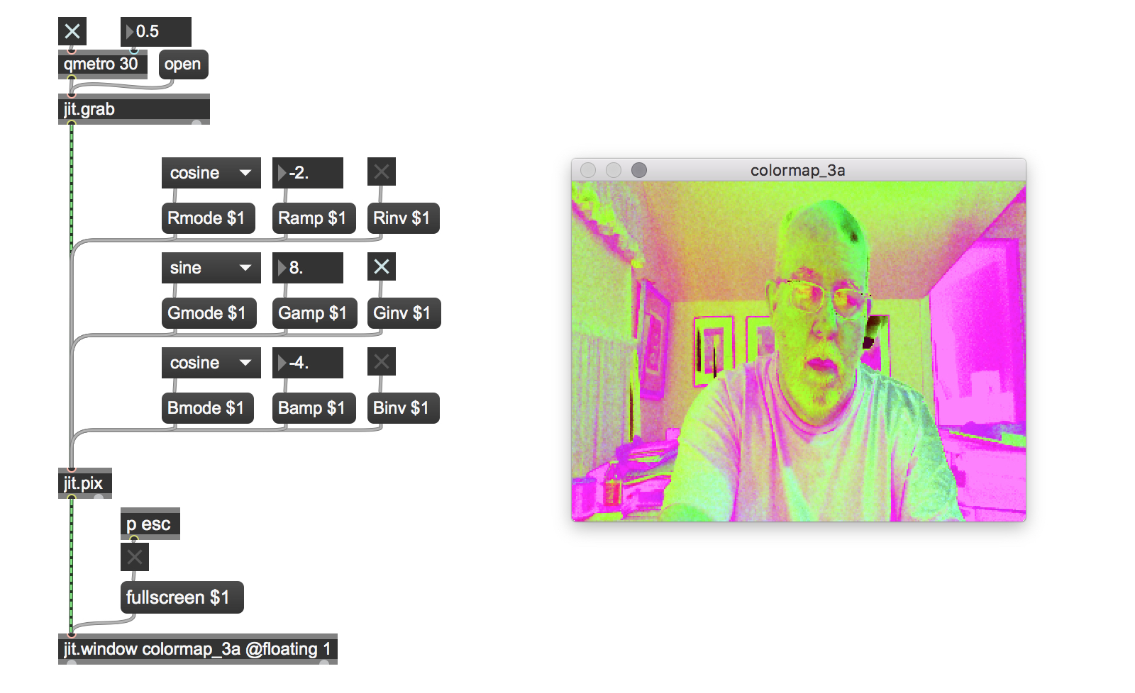
We’ll also add two more mapping choices: mapping using a sine function, or performing no calculation at all and simply passing the original color value. As a final finishing touch, you’ll be able to invert the output for the red, green, and blue planes. This patch is perfect for those Richard Avedon solarized Beatles portraits you’ve been thinking of trying to duplicate:
Here’s a look at what’s inside the colormap_3a patch’s jit.pix object:
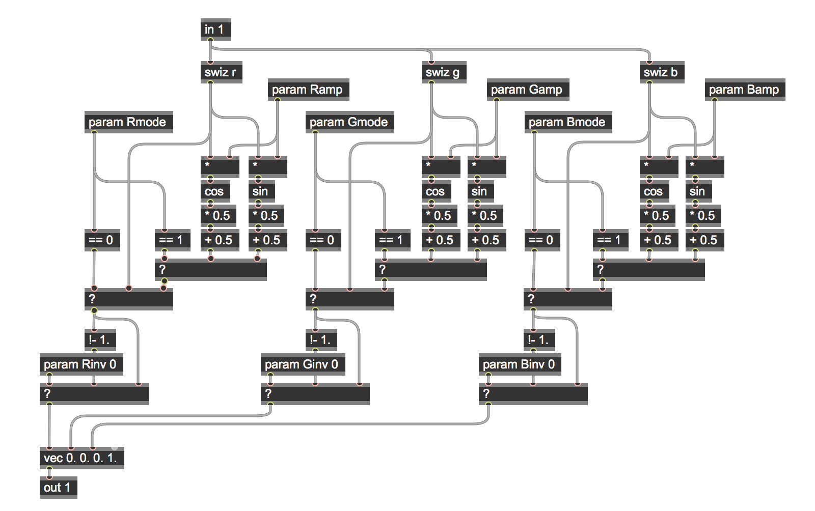
You’ll notice that the patch is composed of three sections, each of which has a swiz operator at the top. When a new matrix/vector arrives in the in 1 input operator, the red, green, and blue values are unpacked/swizzled. Each of these values is a floating-point number in the range 0. – 1.0, and the three portions of the patch process each color value independently of the others using the same logic you’ll recognize from our last patch.
At the very bottom of the patch, you’ll see a vec operator. As with other Gen operators, the number of inlets it has will depend on the number of arguments (default values) typed into the object box when you create a vec operator. We’re working with RGBA color values here, so the operator has four arguments. You’ll also notice that only three of the inlets of the vec operator are connected elsewhere in the patch. That’s because we aren’t doing any alpha channel processing in this patch, so all we have to do is to provide a default value of 1.0 as an initial argument for the fourth (alpha channel) inlet.
All we needed to do to accommodate the additional channel processing was to change the names of the param objects when we duplicated the functionality from our earlier tutorial patch. So we now choose whether to pass or process the color values (based on the Rmode/Gmode/Bmode parameters), and to choose whether or not to invert the output (based on the Rinv/Ginv/Binv parameters).
Where Am I?
In the xy_swizzle_1 tutorial patch, we’re going to look at another technique: using swiz operators for image compositing.
In the jit.pix 2d image world, the location of an individual pixel is identified by x and y coordinate positions, where x and y coordinates are floating-point numbers in the range 0. – 1.0 (the same value range as our color values).
If you’ve taken a look at Andrew Benson’s tutorial on the jit.expr object, then you already know that you’re dealing with what we called normalized numbers. Jitter Gen objects work with them when you want to work with object position by means of the norm operator (which provides a way to access the normalized coordinates of an input matrix) in conjunction with the sample operator, which lets us access vectors from another cell in our image.
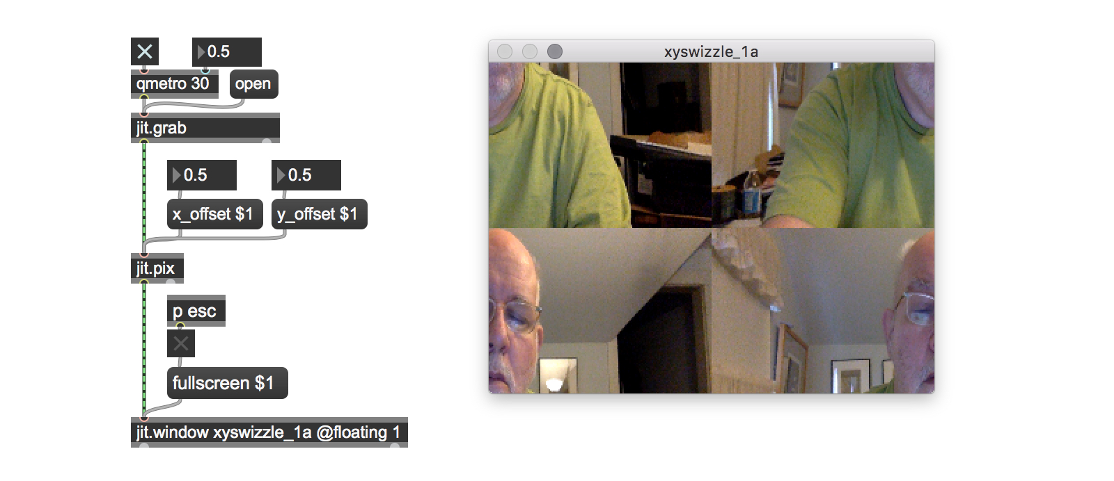
Here’s a simple patch that shows how swizzling position values works:

The input vector from the in 1 operator is sent to the sample operator, whose right-hand input takes a vector as input containing the x and y values that specify a horizontal and vertical offset from the norm value on which we’re performing the operation. Sending a vector containing a pair of zero values would sample the same cell as our input and pass it to the output.
In order to set offset values and construct an offset vector, we use the norm operator to provide us with x and y coordinates in the range of 0. To 1.0. The swiz operator returns the current x and y coordinates for each of the cells in the input matrix (the default is the location of the cell we’re working on). When we add some value to the swizzled output values for x and y, we are going to sample another cell offset from the original input – adding an x offset value of .5 to the swizzled value will locate a cell which is half the length of the input matrix to the right. Similarly, a y offset value of .5 will locate a cell which is half the height of the input matrix down (negative floating-point values indicate offsets up/to the left). Feeding that value to the sample operator will fetch the vector values for that cell (alpha/red/green/blue) and output them.
You might wonder what will happen if the sum of the norm value and the offset value is less than 0. or greater than 1.0. It’s not intuitively obvious from the patch, but the Jitter Gen sample object automatically wraps any input values which are not in the expected range to keep all of our sums safely within bounds. We’ll make use of this feature of the sample operator again later in this tutorial (and introduce another way to handle data mapping in our Tutorial 2b).
The visual result of this is that the displayed image will appear to “scroll” horizontally or vertically.
Mirror, Mirror on the wall….
One interesting feature of working with the 0. – 1.0 floating point data range is that we can make modify data within that to reflect our image on the x- or y-axis. This simple observation forms the basis for the xy_swizzle_2a tutorial patch, which uses the swizzled x and y values and offsets to create a simple kaleidoscope effect. To achieve this effect, we swizzle out the x and y position values, give them an offset, and then use the offset values to mirror the input horizontally and vertically.
The patch contains four sections that handle each of the image rotations.
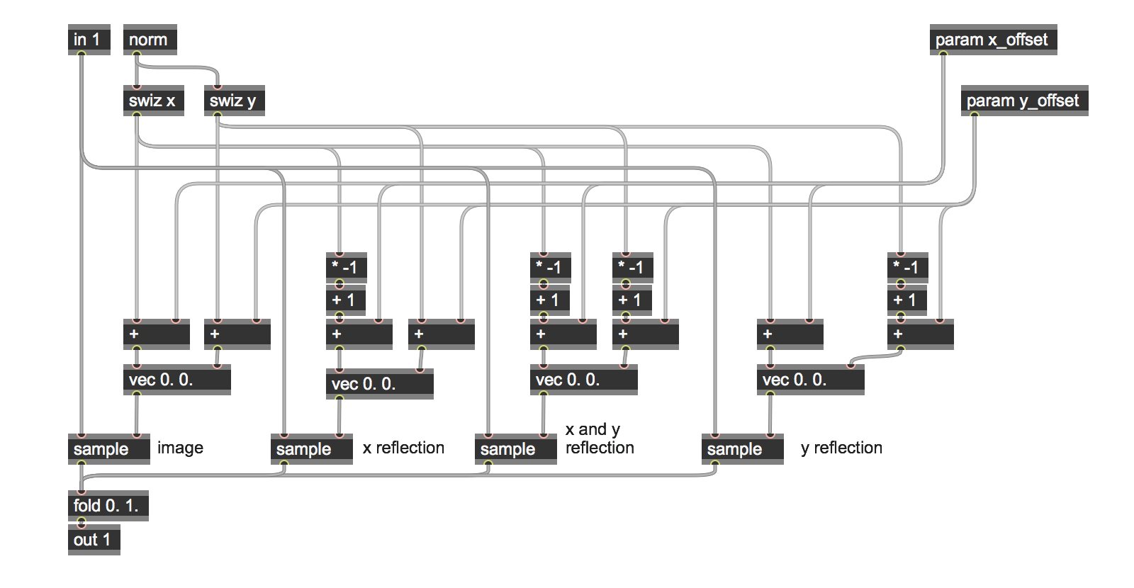
How is it that we can get those multiple sampled values to be applied to each individual cell? The Gen patch simply adds the swizzed vector values for x and y and their respective offset values together.
In those cases where we want to reflect our vector with respect to the x or y axes, we use a combination of a * -1 and a + 1 operator. As before, the Jitter Gen sample object automatically wraps any input values for the sum of the norm and offset values.
Of course, adding those four vector values together might also exceed a value of 1.0, so a little housekeeping is in order here, too. We could multiply each of the sampled vectors by .25 and then add them together, but I wanted to take another opportunity to remind you that there are other interesting ways of getting interesting effects. The tutorial patch does something easy that produces nice results: we sum all four results together and add a fold 0. 1. operator to keep the color values in their proper range.
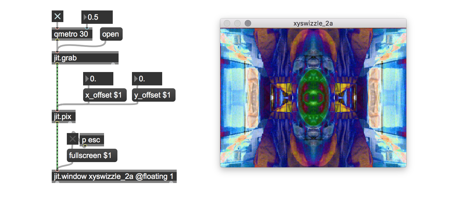
Finally, the swizzlemap_1a tutorial patch unites color mapping and image compositing for subtle and enjoyable visual effects.
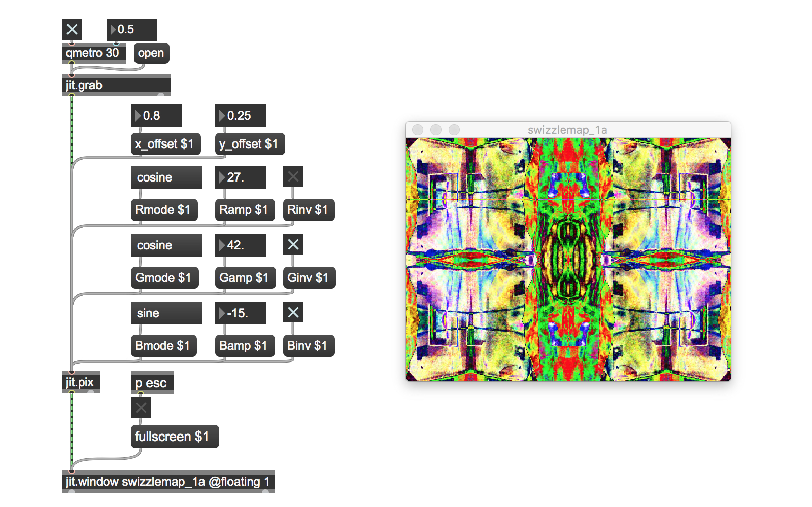
I hope this little collection of patches has given you a reasonable place to start in your exploration of the riches of the Jitter family of Gen objects. Now that you’ve finished with tutorial 2a, take a break. Meditate, feed the cat, eat a candy bar, read a sonnet, or have a pint of the foaming beverage of your choice. After a short break, dive right into tutorial 2b.
We’re going to take what you just learned in these patches and show you a better way – we’ll rewrite them to make proper and more efficient use of the Jitter Gen environment by using vector expressions. It’s best to dig in while what you’ve just seen and learned is fresh in your mind.
by Gregory Taylor on February 2, 2012

