Winter's Day gen~: The Wavetank

The ZenSlap, in whatever form, shakes together pre-existing knowledge in the recipient's head, so they see what they (in principle) already know but didn't see. The right slap can bring two thoughts together that had been sitting next to each other, but unconnected, for a long time... or a set of thoughts needing only one more to make a complete set. At the wrong time, a slap (finding only the one thought) only hurts. The art of the master is to recognize when the thoughts are there.

On A Winter's Day....

So I’m sitting at my desk practicing trying to “empty my mind and think of nothing” on a Wisconsin winter day. The sun’s out, but not heating things up all that much, and I’m having trouble thinking of nothing. Instead, I’m idly glancing around my workspace when my eye falls upon my Eurorack setup. I’ve just taken all the patchcords out, figuring that nowhere might also be a good place to start when Euroracking, too.

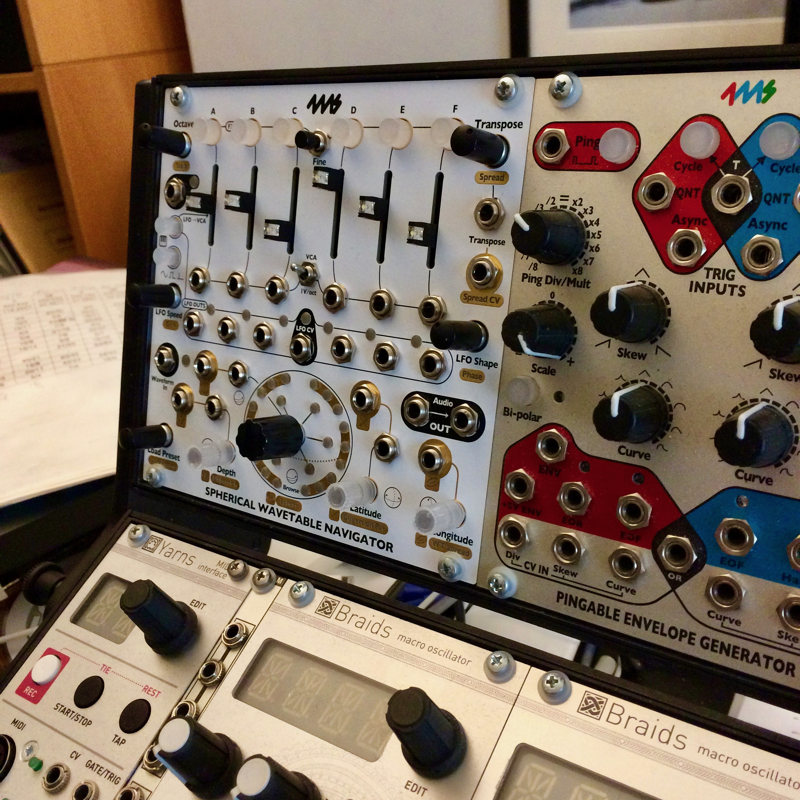
My eye falls on the snowy white front panel of the 4MS Spherical Wavetable Navigator in my rack, and I start wondering about that module. Without warning, I suddenly find myself thinking about gen~ patching.

That’s how it started.

When I got the module, I spent quite a lot of time just modulating the controls for the module and trying to make some sense of the results. That afternoon, I found myself thinking about doing a little wavetable-based gen~ patching that might duplicate or somehow mirror my hours of modulating Eurorack fun.

To refresh my memory, I decided to download the module’s manual and read about how the 4MS folks conceived of the design. That, in turn, pointed me to their SphereEdit (available for Mac or Windows) application and a nice collection of wavetables. While the manual was clear and helpful, although I guess that the idea of a sphere was metaphorically challenging. In a flash of insight, I realized that I ought to be thinking about interpolating and folding as well - and suddenly things kind of fell into place. I started thinking not of a sphere, but of an Escheresque apartment building whose stairs to the roof left you on the first floor, and….

The more I thought about it, the more I thought it’d be interesting to try implementing the idea in gen~ at single-sample accuracy using the wave operator. Since I um… work slowly (Yeah, that’s it. I work slowly), I thought that I’d start with something modest based on that white-panel SWN module sitting over there in my Rack.

Let’s work with one set of wavetables, and just set up a simple readback and experiment with a little modulation and see how that goes.

This is the record of that idea. To be honest, the duration was more than a winter’s day, and - now that it’s working - I think I have some more enjoyable days ahead, too.

Note to Ableton Live Suite users: Access to Gen requires a full Max license. Get details on crossgrading!

The Basic Idea

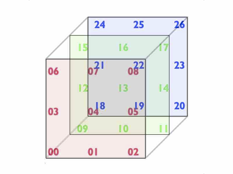
Okay. Imagine that you have 27 waveforms arranged as a “cube.” You have three "stacked" 3 x 3 matrices of waveforms. The output sound will be the result of mixing together three sets of interpolated waveforms, based upon the horizontal (X), vertical (Y), and depth (Z) position in the cube at any given time.

This idea goes in all kinds of interesting directions. For one thing, any new trio of 3D values will result in a unique waveform. In addition, if that trio of values is generated as a result of some kind of movement, the output will smoothly crossfade from one waveform to the next - you can modulate one axis to interpolate horizontal, vertical or depth-based modulations, or as many as you’d like. You can use time-repeating algorithms to modulate your waveforms relative to each other, experiment with different ways to describe trajectories inside of the “cube,” and so on.

Some version of this idea is in play all over the current landscape of wavetable synthesis - from the Eurorack Spherical Wavetable Navigator that started me thinking about this in the first place to the lovely Morphing Terrarium or current keyboard synths such as the Hydrasynth, the Argon8, or the new Korg Wavestate.

Starting Out

The Spherical Wavetable Navigator manual gave me a description of the wavetable files I'd be working with - the files intended for reading into the Eurorack module’s buffer were composed of some number of single-cycle waveforms, laid end-to-end. Each of those single-cycle waveforms is going to correspond to one of the waveforms that make up the “cube” (or, as the Spherical Wavetable Navigator calls it, the “sphere”).

I think it’s easier for me to use the cube as a metaphorical starting point, with the additional notion that you can think of each single-cycle waveform in the cubic arrangement as a room — where each wall and floor between the single-cycle waveform rooms is acoustically transparent, and every wall/floor/ceiling has the same sounds in their corners as well.

Since I was going to be interpolating among the single-cycle waveforms in the file, I needed to have a way for my gen~ patcher to load a buffer operator and figure out a way to identify the start and end points of any of those 27 single-cycle waveforms in the file, sample by sample.

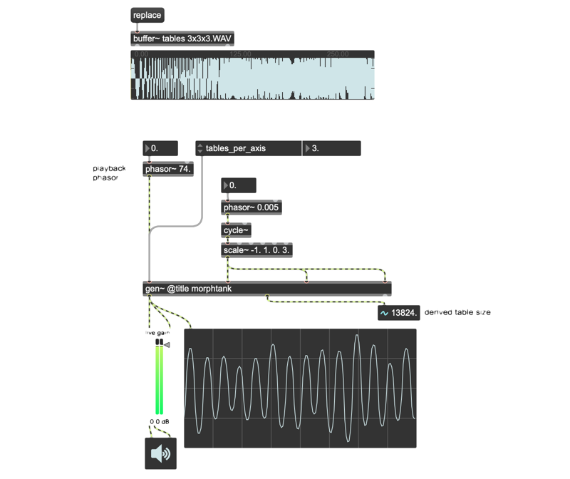
Happily, the buffer operator will, when loaded, start broadcasting the total number of samples it contains. I know that I want my “cube” to have three different waveforms along each of the axes in the cube, so this little bit of gen~ patching lets me set a parameter for that number of waveforms along each axis, and then to cube that number and calculate how many samples will be in each single cycle waveform:

Since a bunch of the calculations I’ll be doing requires that number of axes, using a param operator lets me use that value throughout my patch. In addition, storing that number of samples in each of the 27 waveforms using the history operator will also let me use that value later on, as well. Now that I’ve got a way to determine who many samples constitute a single-cycle waveform based on the length of my buffer and the number of waveforms, what does playback look like?

The file 01_Wavetable_play_patch shows a simple but diverting example of selectable playback using the gen~ wave operator.

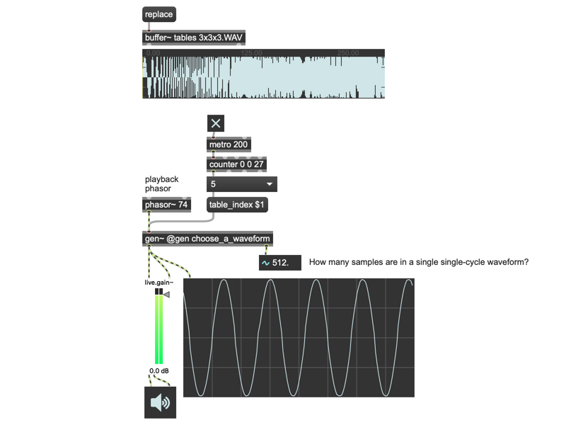
Let’s take a look inside the gen~ patcher choose_a_waveform:

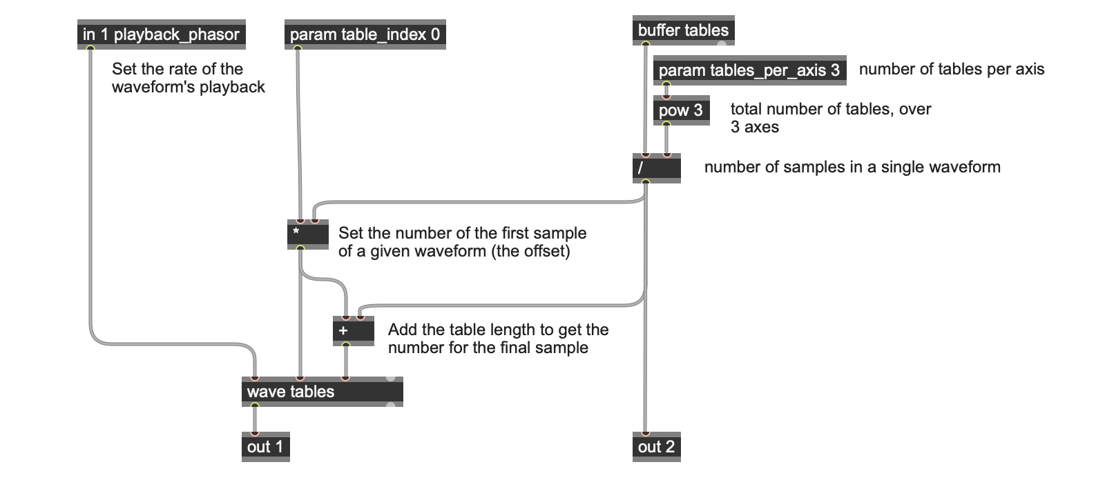
You’ll quickly recognize the same buffer operator-based patching we just used to set the length of a single-cycle waveform in samples. Once we have that number and we know the number of waveforms in our file (27). Then it’s easy to specify the values that correspond to the start and endpoints of our single-cycle waveform (which is what the wave operator needs as its second and third inputs): We take a value between 0 and 26 (the table_index parameter) and multiply it by the number of samples in each single-cycle waveform to get our starting point. Adding that same number again gives us the endpoint sample value. We use a phasor~ object in the parent patch to control the playback rate. For extra fun, the patcher choose_a_waveform patcher uses a standard Max metro and counter object to automate stepping through the waveforms in the file.

Moving in 3D

Now that we know how to divide my buffer into the right number of N-sample chunks and to select the waveform I want to play, it’s time to think about what moving between waveforms in my “cube” actually entails.

For each of the three positions that describe the “space” in my cube, I’ll have three versions of the same thing: I’ll be interpolating between two waveforms for each of the X, Y, and Z coordinates. And then interpolating all three of them together.

So that means I’ll need three values in the range of 0 - 3.0, and - since I’m interested in interpolating at the “edges” I”ll need to be able to wrap values at the minimum and maximum of the range.

Let’s look at the layout of our single-cycle waveforms again:

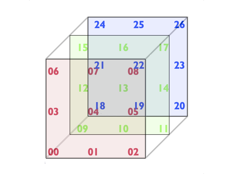
• Interpolation along the X axis moves between waveforms 0, 1, and 2 or 12, 13 and 14 (in the second “plane”, 24, 25, and 26 in the third “plane”, etc..

• Interpolation along the Y axis moves between waveforms 0, 3, and 6 or 9, 12 and 15 (in the second “plane” 20, 23, and 26 in the third “plane”, etc..

• Interpolation along the Z axis moves between waveforms 2, 11, and 20, 8, 17, and 26 (in the second “plane”, 6, 15, and 24 in the third “plane”, etc.

The summing of the axis-to-index inlets is crucial, and the way we connect 1D space (the set of wavetables in the buffer) to a 3D space bears a little more explanation.

As in the example above, when we think of the X axis of our collection of waveforms, the wavetables are end-to-end, with a spacing of 1 (e.g. 0, 1, and 2). Since our tables_per_axis = 3, that means the axis requires 3 wavetables.

When we think of the Y axis, we have to then jump every 3 wavetables (to give space for the X axis). Moving 1 step through Y means jumping over 3 wavetables (e.g. 0, 3, and 6). So we end up needing 3x3=9 slots to cover X and Y.

In the the Z axis, we have to then jump every 9 wavetables (to give space for the X and Y axes). Moving 1 step through Z means jumping over 9 wavetables (e.g. 0, 9, and 18). So we end up needing 9x3=17 slots to cover X, Y and Z.

The lion’s share of my time in patching this involved trying to puzzle out how to translate three values in the range of 0 - 3.0 so as to come up with the two waveforms I wanted to interpolate between (i.e. to identify the start and endpoints as sample numbers) and the interpolation value between the two waveforms to be applied to them, and then to come up with a way to mix those three separate results.

That’s what the gen~ wavetank patch does.

It looks sort of complicated, but I’ll break it down into the individual pieces and walk you through them.
You’ve already seen how we can derive the sample length of waveforms on load, so let’s move along….

Axes To Indices

First, we need to have a way to convert one of the X, Y, or Z values into information about waveform numbers and interpolation amounts for our 3 x 3 x 3 cube of waveforms. The three axis_to_index patchers take care of that for us.

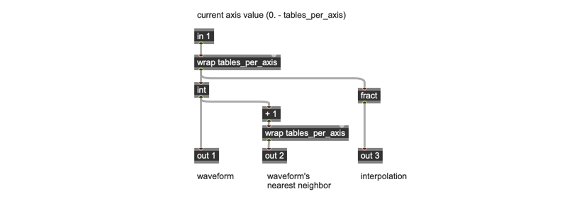
Each axis_to_index gen patcher takes a continuous index value as its input. You’ll notice that we’re making use of the tables_per_axis parameter we use in the parent wavetank patcher for calculating the length of each individual waveform in samples. That value shows up in this patcher because we need to specify that any value we receive in the patcher’s input will be properly wrapped to be in the range of 0. – 3.0

Once we wrap the X, Y, or Z input value, we convert it to two integer values that specify the two nearest neighbors in our sequence of waveforms by converting the axis value to an integer and adding 1 to it, and using the tables_per_axis parameter once again to make sure we wrap the nearest neighbor back to 0 if the current integer value is 3.

So we’re ready to begin reading from our file full of waveforms. But remember – that file full of waveforms is a linear group of single-sample waveforms. How do we decide what the sample offset to start reading for any of our 27 waveforms is?

We need a way to take those nearest neighbor integer values from the axis_to_index gen patcher and to scale them up to corresponding offsets in the wavetables file. Once again, we can use the tables_per_axis parameter to help us out by multiplying the two index integer values by 0 (which always gives us a value of 1.), 3 (1 * the number of tables per axis) and 9 (the tables_per_axis value squared).

We’re now ready to start reading from our buffer full of waveforms!

By the way – you might have been reading along and sort of wondering why I bothered to create a parameter that described the number of tables per axis for this patch instead of just plugging in a 3 everywhere I need to reference the number of tables per axis. You see that sequence of multiplication operators in the wavetank patch (* 1, * tables_per_axis, and * tables_per_axis * tables_per_axis) that we use to get the 1, 3, and 9 values we use for the waveform offsets. It turns out that using a param operator to hold that value here and elsewhere is going to let us do something really cool later on. Stay tuned!

Reading the Wavetables File

The middle of our wavetank gen patcher is where we really get down to the business of reading values from our buffer full of waveforms and then creating the audio output. One thing you’ll notice is that we’re using the playback phasor (inlet 1 in our wavetank gen~ patcher) to set the rate at which we read and write samples. But why are there four read_the_wavetable gen patchers? And – more to the point, why are they reading from the buffer twice in each of the read_the_wavetable gen patchers, for a total of eight wavetable readers?

The answer has to do – once again – with that question of dimensionality.

Let’s start with a simple case: if you’re using a crossfader in your DJ rig, you’re mixing in 1 dimension. You need two sources (or two wavetable readers) to handle the crossfade between input 1 (call it A) and input 2 (call it B).

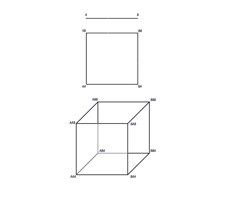
Now, suppose you want to mix in two dimensions. It’s a square instead of a line, and your square has 4 corners, so you need to double what you had in the single dimension – a pair of sources for each A and B (AA, AB, BA, BB).

But we’re wanting to mix in three dimensions, which means we’re dealing with a cube instead of a square, that means we need to double the number of sources again (AAA, AAB, ABA, ABB, and so on), giving us eight sources.

So – for N axes in the space we’re trying to mix in you need 2^N (2 x 2 x 2 =8) sources to mix. A line has two ends, a square has four corners, and a cube has eight corners. Presto – eight wavetable readers, organized as four groups of two (That means that your hypercube mixing wavetank is going to need a lot more wavetable readers - 16 of 'em).

That idea of performing interpolation in three dimensions on data is something that folks in the graphics world do pretty commonly – it even has a name: trilinear interpolation or box interpolation. One place you’re likely to find it in use in the graphics world involves doing lookups in a 3D texture or a voxel grid. For more information on trilinear interpolation, Paul Bourke’s website has a great page on interpolation methods you might even want to bookmark. The page is here — scroll down to the “Trilinear interpolation” section.

And yes, this is the same Paul Bourke whose collection of code for Chaotic attractors is the site I’ve directed anyone nearby who would listen. Paul’s site is a fount of knowledge and clarity.

Now that we have an idea of why we need all that wavetable reading done and why we need to mix and interpolate information for all three axes, let’s look inside the read_the_wavetable gen patcher.

First, you’ll notice that we’re using the same patcher for each of our four pairs of buffer reading we’re doing, and that each and every single one of the read_the_wavetable gen patchers is using the wavetable phasor in the main patch to control the rate at which it’s reading and writing values (the in 1 operator).

Remember those three index values (two integers and a floating-point interpolation value) we got from the axis_to_index patcher and scaled up using the tables_per_axis parameter value? Those are represented by in 2, in 3, and in 5. The integer index values of in 2 and in 3 are the “nearest neighbor” values that we’ll use to set the start and the endpoints we’ll need when reading from our buffer. We get those start and endpoints by using the table_length parameter that corresponds to the number of samples for each individual waveform in the wavetable file. We calculated that value when the buffer was initially loaded. The table indices (multiplied by 1, 3, or 9) are multiplied by the table_length variable to get the initial offset into the buffer, and the endpoint is the sum of that offset plus the table length.

The gen~ wave operator handles the buffer-based wavetable reading. At the rate set by the phasor waveform input, it samples from the buffers at the specified locations, and then mixes the two outputs based on an interpolation value.

This same sequence is repeated for each of the other three read_the_wavetable gen patchers, which are, in turn, to achieve the desired 3D waveform result.

A Question of Scale

Once I had all that wrapped up together, I had the patch you'll find in the tutorial patches folder called 02_Wavetank_3x3x3. I could now grab the audio files from the SphereEdit application and play load and go....

But remember my earlier comment about deciding to set the number of tables for each axis of my wavetank using the tables_per_axis parameter rather than salting my patch with the number 3?

Going the parameter route allowed me to do something super cool. Suppose I want to work with a collection of sixty-four single-cycle waveforms — a 4 x 4 x 4 cube instead of 3 x 3 x 3. There are a whole lot of wavetable files out there in that form (these, for example). What kinds of modifications do I need to make to my patch?

None. Zip. Zilch, Nada.

All I need to do is to set the value of my tables_per_axis parameter to 4 instead of 3 (with the help of a handy Max attrui object) and I’m ready to go. The patching subtleties of working with the larger cube (with a new excursus value of 0. - 4.0 which will be automatically set, by the way) are exactly the same.

I’ve included a file of 64 single-cycle waveforms in the downloadable folder (PPG_WA00.WAV) for you to try, and I'd suggest that you head over to the Synthesis Technology WaveEdit online page to download a whole bunch of lovely 64-waveform files.

All you need to do is to change the tables_per_axis parameter and read in a new file.

You’re welcome.

All Mod(ulations) Cons(idered)

Once I had my gen~ patch working, I decided to spend a little time exploring. I’d be lying to you if I didn’t just own up to the fact that there was some space between the understanding of the gen~ patch before me and what I heard. In the interests of getting more of that knowledge into my head through my ears, I put together a simplified version of my patch (the 03_Wavetank_starter_patch) that let me manipulate each of the X, Y, and Z axis values manually (I even decided to try it using my newfound 4 x 4 x 4 cube, just for fun).

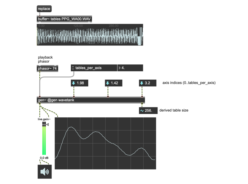
It worked great - I could quietly commune with the patch and exercise each axis value for my cube individually and get a sense of the relationship between modulating the X, Y, or Z axes individually, and combining them.

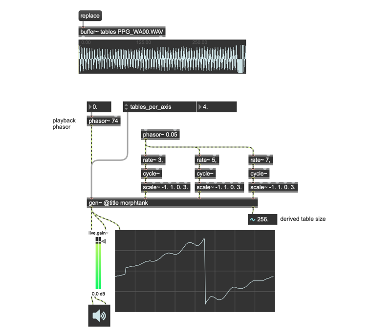
After that, the next move is obvious — modulate those axes! And thus, the 04_Wavetank_EZ_rate patch was born. Nothing special here. Just a couple of rate~ objects to set up a sequence of sine waves (phasor~ > rate~ > cycle~) for modulating fun.

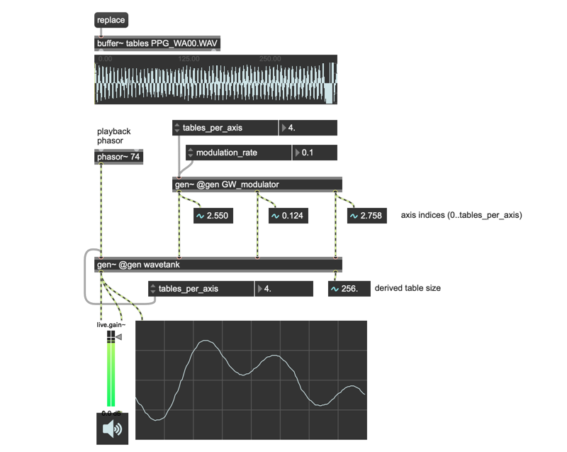
There are all kinds of modulation possibilities, obviously (3-output chaotic attractors come to mind, for example….). But I’d like to share something in the 05_Wavetank_GW_modulation patch from my friend and colleague Graham Wakefield (Graham is the man who gen~ calls “Daddy,” in case you didn’t know).

I was in touch with Graham in the course of developing these patches. At one point in our correspondence, he sent me an explanation/suggestion that included the gen~ patcher that appears as (GW_modulator).

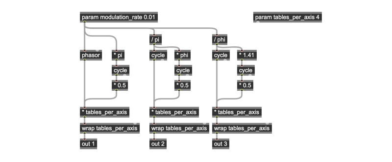
It included some clever patching making use of two of the numerical constants that Gen includes — Pi and Phi. He was pretty humble about it, claiming that he “just wanted something that wouldn’t repeat”; Since Phi and Pi are transcendental numbers, they have no simple ratios with other numbers.

I’ll let you explore the behavior of this elegant little hack yourself - just load a wavetable file, make sure that the tables_per_axis values are set for the file you read in, set the modulation_rate value to something sweet and slow, and settle back to enjoy.

Quo Vadis?

I started out talking about inspiration and enlightenment. While it’s common to hear people talking about inspiration as though the relation between the idea that set things in motion is somehow completed in a given instance of what results from that initial idea, that doesn't feel like that's the case here. I look and listen and imagine what might be next.

And - for me - the next isn't necessarily a case of trying to slavishly emulate my Eurorack module. I’ve only ported a small portion of the Spherical Wavetable Navigator’s functionality, but as the wavetank cycles quietly in the background, I find myself thinking along very different lines, and already wondering how I can use gen~ to follow those lines of thinking. Feel free to share where this bit of gen~ patching may take you, and happy patching!

I am very grateful to Graham Wakefield for his patience in giving me the right metaphors by which I could start unravelling the idea of trilinear interpolation, as well as for his lovely Pi/Phi nonrepeating modulator hack. He shreds and rules.