An MC Journey, Part 4
Welcome to the next part of my MC journey. As I said when I started this trip, it was personal. While I love opening other people’s patches and twiddling the knobs and adjusting the sliders and enjoying the results, I’m usually in search of some sort of inspiration that I can yank sideways into the place where I work.
For this "step along the way" in the MC journey I thought I'd show you another real-world bit of MC patching that takes a number of past projects/tutorials I've created and combines them with what I've learned during this series to make something that I (at least) find interesting and useful.
As I said earlier on, I'm generally not someone who's necessarily moved by MC's ability to control very large numbers of things (although David Zicarelli and Tom Hall's appearance at the Ableton Loop event really impressed me and probably got me intrigued in the first place — you really ought to download the patches and watch the video of the presentation!). But there are places where I've listened to something I've made and thought that perhaps the MC functions would let me explore them on a "slightly larger scale."
One tutorial I've recently written for the Cycling '74 website that comes directly out of my own practice and interest set was borne of my interest in exploring the 4MS Spherical Wavetable Navigator and wondering how I might use gen~ to create something interesting. The resulting tutorial — Winter's Day gen~: The Wavetank — led to the creation of a patch that let me load an 3d grid of waveforms that would be traversed to create an output that morphed interestingly.
It was lovely, but I found myself thinking about what MC might do for me there. How about an MC version of that patch whose pitches and X, Y, and Z traversal values could be independently controlled?
I've also been really interested of late in chaotic attractor equations what I could use in places where a simple LFO wouldn't get me the kind of slowly changing outputs that seemed more to me like "intentionality." I found myself wondering what use I might make of patches like this. Since chaotic attractor patches are heavily dependent on the initialization values (and not all possible values are created equal when it comes to chaotic behavior), any MC versions would start from precisely the same place — I'd need to think about spreading out the results in time or modifying them in some other way.
The value of my careful and pretty personal perusal of MC features (see the previous installments in this series) also gave me a pretty clear idea of how I might approach this. This tutorial is a walkthrough of using MC to realize those ideas.
A Little Time In The Tank
The morphing wavetank I created in the Winter's Day gen~ tutorial is an idea that’s stuck with me since first I started twiddling dials on the 4MS Spherical Wavetable Modulator Eurorack oscillator and wondering whether I could use gen~ to do something similar.
If you’re interested in the gen~ patching that underlies how it’s done, I’d recommend you take a look back at the original tutorial. Simply put, I created a patch that let me take an audio file composed of a specific number of single-sample waveforms and create a cube (3x3x3 or 4x4x4) I could traverse in 3D using three parameter values to represent a height, width, and depth location within the cube. The resulting outputs was an interpolated result derived from the 27 or 64 waveforms. By modulating the X, Y, and Z parameters, I could produce an interesting morphed output — particularly when driving those parameter values using a set of LFOs.
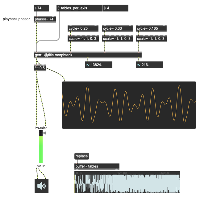
On reflection, the MC toolkit suggested some really interesting possibilities:
I could use MC to create multiples instances of the morphtank patcher tuned to different frequencies — chords, harmonic multiples, etc.
I could also create some patching that would change the X, Y, and Z inputs for the morphtank patcher at different rates, from different offsets, and so on. That might be cool even if all the morphtanks were running at the same base frequency!
I could use MC tools to spatialize/control those multiple outputs.
In short, it was a perfect candidate for my next MC project.
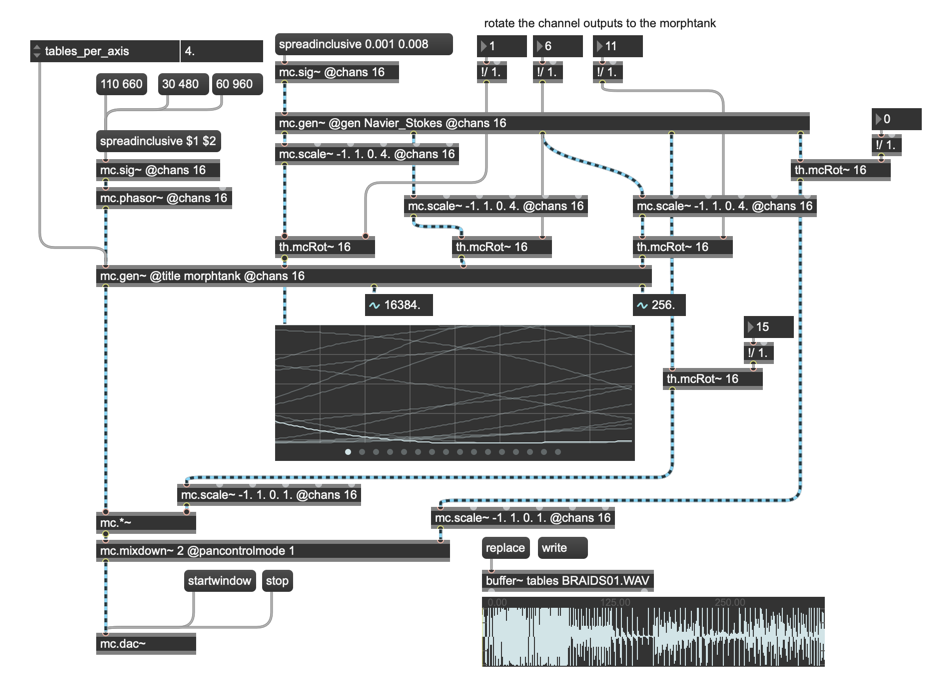
Creating the MC patch was simple: just add an mc.gen~ @gen morphtank @chans 16 object to my MSP patch. Presto — 16 morphtanks ready to go!
There were a couple of things that I wanted to keep for all 16 instances — the control of the audio files used for the wavetank and its parameters. But when it came to setting the base frequency for each of the 16 morphtank patches, my MC investigations gave me two attractive options:
I could use a harmonic (or subhamonic) 1 <frequency> message connected to an mc.sig~ @chans 16 object to set my instances to frequencies based on the harmonic overtone series.
I could also use the spread messages in combination with an mc.sig~ @chans 16 object to distribute the base frequencies of each instance across a linear frequency range I could specify.
Based on my MC journey, I opted for the second approach, since I realized that the spreadinclusive message that I'd investigated in Part 1 of this series combined with an interesting frequency range could produce some interesting and dense “chords.”
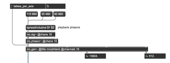
Dealing with the outputs was just as easy, but I need to talk a little about using my chaotic attractor patch first. I’ll come back to that in just a bit.
Chaos On The Faders
In my initial explorations of the morphing wavetank, I'd either manually adjusted the three sliders that set the "position" in the cube I wanted to interpolate waveform output from, or I connected up some LFOs with their outputs set to a 0.0 - 4.0 range to animate things automatically.
But the more I listened to the LFO results, the more I thought about what I might use for a little more complex X, Y, and Z parameter input. It might have been the result of my using a single LFO with rate~-driven outputs that modulated the three parameters in cyclic fashion that started me thinking in this direction, or the more simple observation that I don't play faders "like they're LFOs" when I perform.
In any case, that insight got me thinking about using Chaotic equations as modulation sources; they generally appeal to me because there is a kind of trajectory to their outputs that is neither "random" (which I certainly am not) nor periodic in the way that an LFO is.
And as I said, the attractors have been an interest of mine for a long time. The very first Gen patch-a-day feature we did back in 2012 included an example I figured would be perfect for use — a trio of patches that implemented a Navier-Stokes equation in three different gen~ formats (a gen~ operator version, a gen~ expr operator version, and a codeboxed version). You'll find it on day 14 of the Gen patch-a-day series.
Here's the original gen~ patcher:
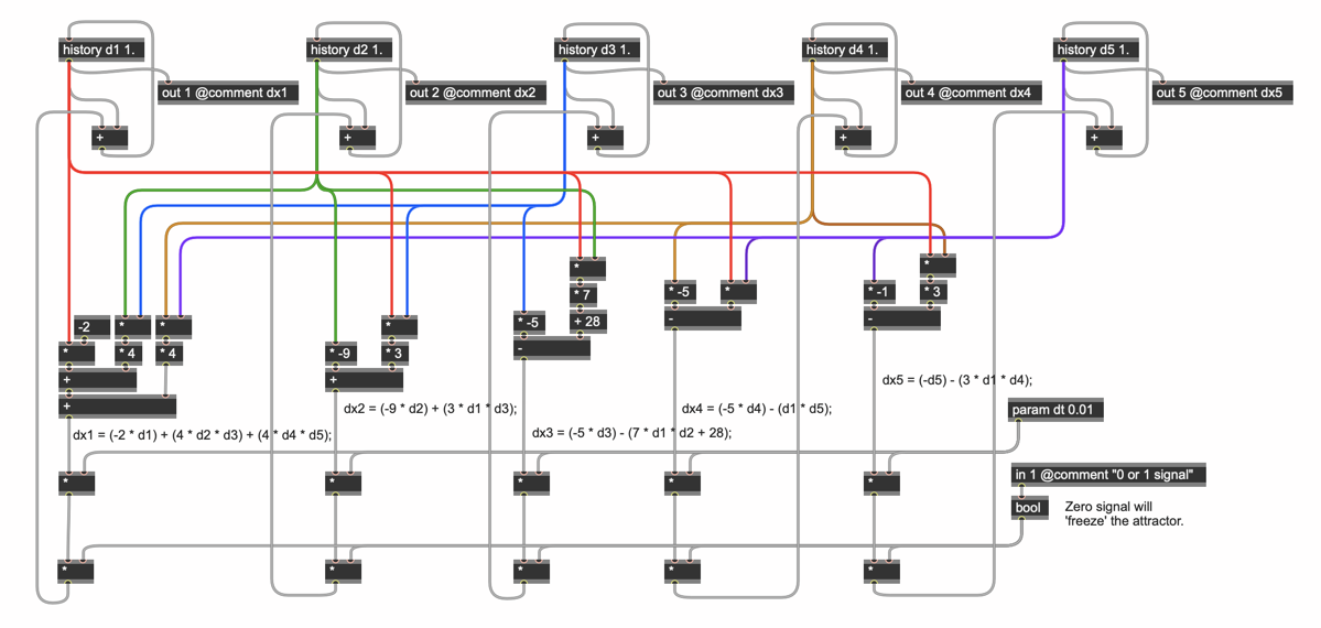
It's an old patch, and the intervening time has led me to reconsider how I'd implement it:
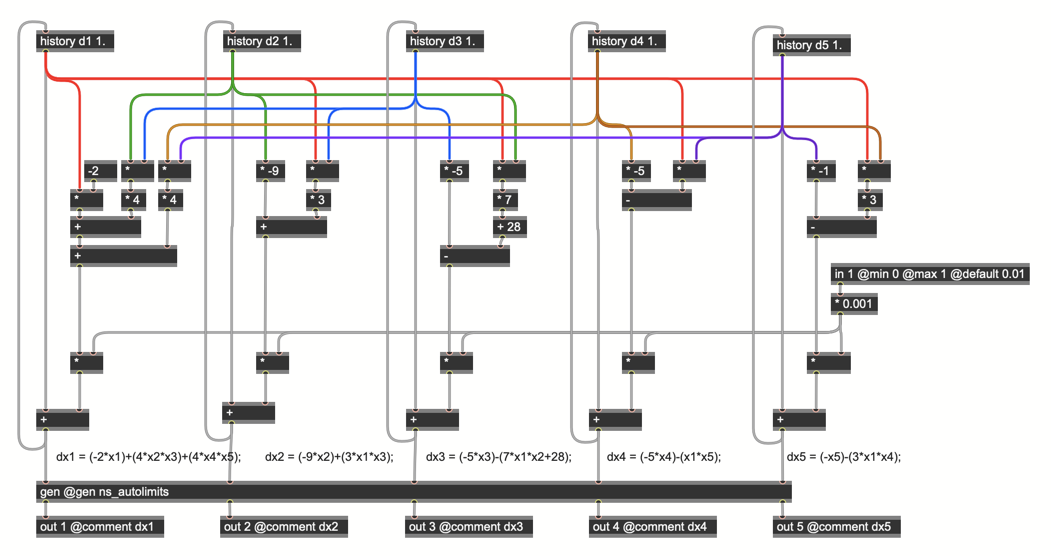
Instead of using a train~ object's output to drive the attractor, I've opted instead for a version of the patch that's "always on." With each tick of gen~'s single sample clock, the attractor calculated the next iteration of itself, and then multiplies the result by a very small value that provides the "rate" at which the attractor runs. That small value is then added to the previous one and stored in a history object. The result is a smooth output at a widely variable range. Turning the attractor "off" is a simple matter of setting the dt (change in time) parameter to a value of 0. And the attractor can be restarted at any point by sending the gen~ object the message restart, which resets all the history objects to their initial state.
Here's the improved version:
Setting Limits
The other change in my gen~ patcher has to do with improvement to the idea of establishing the limits of the attractor's outputs. You'll notice there's a second gen~ patcher added at the bottom there.
In the past, I’d simply coded up the attractor, turned it on and let it run for a few days, and used whatever the relative maximum and minimum limits I had when I stopped the patch from running (we called it “empirical observation”).
However, when I made the switch to the "add a settable increment’s worth of calculation to the previous value" instead of a train-based approach, it occurred to me that I might see slightly different results at different speeds. Since chaotic attractors not only exhibit “sensitive dependence on initial condition” (i.e. you may get very different results depending on the original settings for the initial parameters), it’s also the case that since chaotic equations iterate based on previous values, a single result that varies considerably from the previous one.
This simple change in my gen~ patcher has introduced me to an interesting problem I’m still thinking about: What’s the best way to establish and work with maximum and minimum values when you don’t know what their range is likely to be? Working with chaotic equations generally threw this into sharp relief for me since the behavior of an attractor calculation — in some cases — seemed to produce different results for maxima and minima depending on the dt for the calculation. If I changed the dt value, I might suddenly find that the relative maxima and minimum values changed. I thought that finding a way to smooth that change over time might be the best solution.
Then I remembered George Lewis talking about just this particular kind of problem with respect to his Voyager program during an interview I did with him earlier this year: He was talking about using “leaky integrators” to manage slow changes in values like this.
Simply put, a leaky integrator is easy to make: Instead of using min and max operators to set and store the relative minimum values forever, you store the next maximum or minimum value when you find it.
But you also add some patching that slowly lowers the minimum or maximum values over time. subtracting very small amounts from the minimum value, as well. This slowly changes the amount of the current maximum or minimum by subtraction that’s stored for the next calculation — it “leaks.” Whenever a new high or low value comes along, it sets the maximum or minimum to that new value and it starts leaking again.
I wasn’t sure that I’d have this particular problem at different dt rates, but I thought it’d be best t be cautious, so I mocked up this version for my patch:
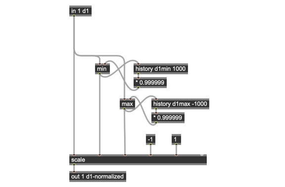
It seemed like a good idea at the time.
Why didn’t I go with that initial min/max > history solution for my leaky integrator? In fact, there’s a very subtle problem with it that didn’t occur to me until my friend Graham Wakefield pointed it out to me; while this solution might work in a situation where the relative maximum and minimum values I’m tracking fall on either size of zero, I’d encounter difficulties in a situation where the relative maximum and minimum both fell above or below zero — the system tends toward zero. The more useful and general case is to create a patch where the leaky integrator’s maximum slowly approaches the minimum in the absence of new maximum values, and vice versa. This makes the patcher more generally useful.
Here’s a version that does just that — the limits now converge on each other by a settable amount (controlled using the param operator and dividing by the current sample rate to get a very small number) to control the rate of “leakage.”
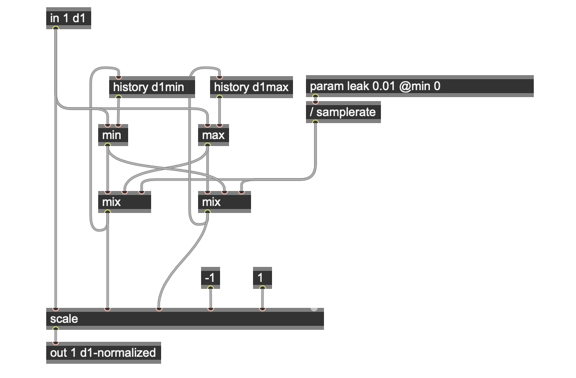
Armed with this new Navier-Stokes gen~ patch, I was ready to start modulating the X, Y, and Z plane traversals for my MC Wavetank.
When it came to setting the rates for the 16 instances, I once again availed myself of the spread messages to set a range for the rate of the attractors' operations.
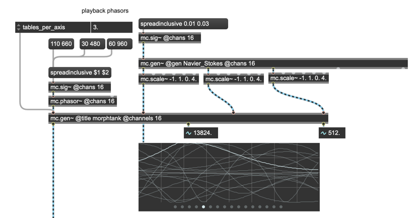
The nice thing about my Navier-Stokes attractor gen~ patch is that it gives me 5 different outlets. I only need three for modulating the Wavetank’s 3d controls, so I started thinking about what else I might do with two more parameters to play with for my 16-channel Wavetank. It wasn’t too hard, really — I thought I’d use one of the leftover attractor outputs to set the output amplitude for each Wavetank channel, and the other one to pan the result across the stereo field.
All of those operations would require scaling the output range of the Navier-Stokes attractor patch’s output: the first three parameters needed to scale the audio range outputs to the 0.0 – 4.0 value I needed for the Wavetank 3D controls, and parameters four and five both needed to be scaled from bipolar to unipolar ranges. Five well-placed mc.scale~ objects took care of that problem with little muss or fuss. After scaling, the Wavetank inputs went straight into the MC version of the gen~ morphtank patch. Similarly, the amplitude was handled by an mc.*~ object.
Spreading It Around
Amazingly, I was very nearly done! All I needed was to set the panning for the 16 individual outputs. Having made my way through the MC panning resources available to me in Part 2 of this series, I knew just how the mc.mixdown~ operator handled panning. I went with mc.mixdown~ 2 pancontrolmode 0 object, which spread the panning out across the stereo field by assigning 0.0 - 1.0 values for left-to-right panning. The fifth parameter outputs from the Navier-Stokes patch (scaled for the 0.0 – 1.0 range) set the panning for each of the 16 Wavetank outputs with a single patchcord connection:
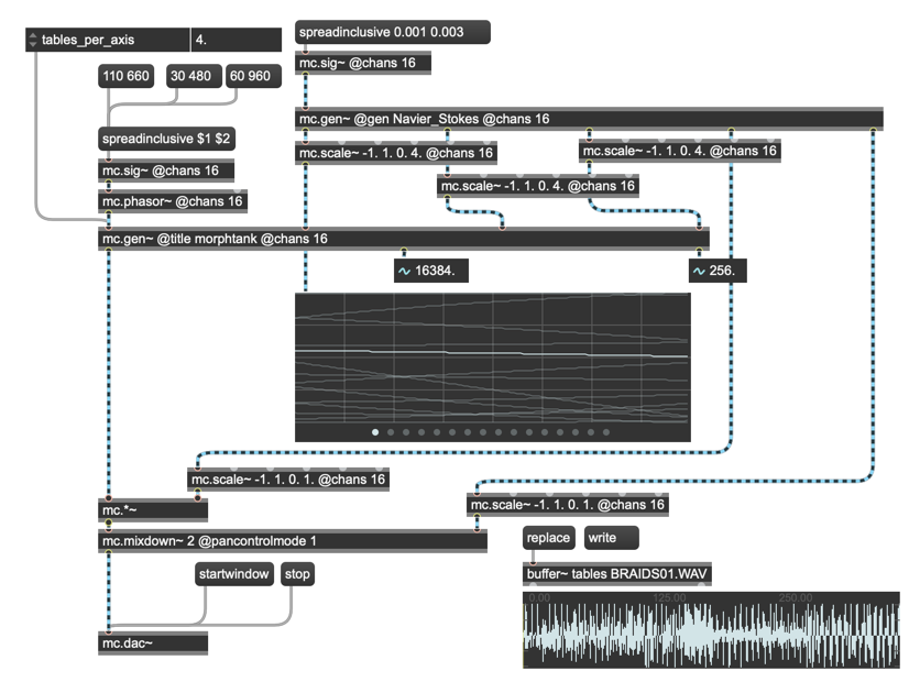
My MC patch was ready for prime time. I turned it on, and... Wow. <Insert some serious tweak time here>
...And One More Tip....
Before I go, I wanted to mention one more little personal tweak that produced some interesting results. As you might imagine, each of the chaotic attractor mc.gen~ patches outputs exactly the same values at the same rates (even though each instance runs at a different rate, the 5 outputs are all clocked the same). I started thinking that a further way to introduce some variety would be to consider "rotating" the X, Y, and Z outputs being sent to the MC version of my morphtank. Since each of the 16 instances would be clocked differently, rotating the X, Y, and Z inputs would mean that each one of them would update at different rates.
So I started researching how I might consider implementing a rotation for those outputs. As I always do, I check the in-app Max help first. There was some discussion about using an mc.matrix~ object, but that looked pretty daunting (and I'm not ashamed to say it). What I did find in the "Search the Forum" results was that Timo Hoogland had produced a suite of MC utilities (available at no cost, although he would appreciate you filling the tip jar, I'm sure) that include an abstraction that does just that. You might want to try it (I obviously can't give you a copy of someone else's work, but here's how I added it the main patch):
Learn More: See all the articles in this series
by Gregory Taylor on June 22, 2021

